Page 188 - Modern Analytical Chemistry

1400-CH06 9/9/99 7:41 AM Page 171

Chapter 6 Equilibrium Chemistry 171

pH p EDTA E

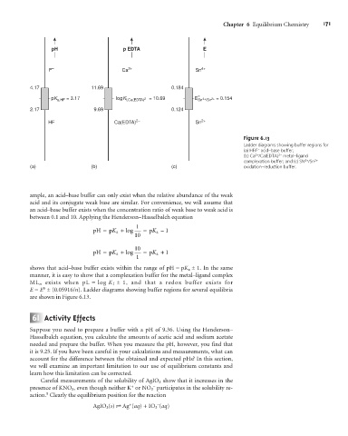
F – Ca 2+ Sn 4+

4.17 11.69 0.184
pK = 3.17 logK 2– = 10.69 E ° 2+ = 0.154
4+
a,HF f,Ca(EDTA) Sn /Sn
2.17 9.69 0.124
HF Ca(EDTA) 2– Sn 2+

Figure 6.13
Ladder diagrams showing buffer regions for
–
(a) HF/F acid–base buffer;
2+
(b) Ca /Ca(EDTA) 2– metal–ligand
4+
complexation buffer; and (c) SN /Sn 2+
(a) (b) (c) oxidation–reduction buffer.

ample, an acid–base buffer can only exist when the relative abundance of the weak
acid and its conjugate weak base are similar. For convenience, we will assume that
an acid–base buffer exists when the concentration ratio of weak base to weak acid is
between 0.1 and 10. Applying the Henderson–Hasselbalch equation
1
K
pH = p a +log = p a K – 1
10
10
pH = p a +log = p a K +
K
1
1
shows that acid–base buffer exists within the range of pH = pK a ± 1. In the same
manner, it is easy to show that a complexation buffer for the metal–ligand complex
ML n exists when pL = log K f ± 1, and that a redox buffer exists for
E = E° ± (0.05916/n). Ladder diagrams showing buffer regions for several equilibria
are shown in Figure 6.13.

6I Activity Effects

Suppose you need to prepare a buffer with a pH of 9.36. Using the Henderson–
Hasselbalch equation, you calculate the amounts of acetic acid and sodium acetate
needed and prepare the buffer. When you measure the pH, however, you find that
it is 9.25. If you have been careful in your calculations and measurements, what can
account for the difference between the obtained and expected pHs? In this section,
we will examine an important limitation to our use of equilibrium constants and
learn how this limitation can be corrected.
Careful measurements of the solubility of AgIO 3 show that it increases in the
+
–
presence of KNO 3 , even though neither K or NO 3 participates in the solubility re-
5
action. Clearly the equilibrium position for the reaction
–
+
AgIO 3 (s) t Ag (aq)+IO 3 (aq)