Page 75 - Modern Optical Engineering The Design of Optical Systems

58 Chapter Four

Thus Eqs. 4.4 through 4.13 constitute a set of expressions which can
be used to solve any problem involving two components. Since two-
component systems constitute the vast majority of optical systems,
these are extremely useful equations. Note that a change of the sign of
the magnification m from plus to minus will result in two completely
different optical systems. They will produce the same enlargement (or
reduction) of the image. One will have an erect, and the other an
inverted, image, but one system may be significantly more suitable
than the other for the intended application.

4.2 The Optical Invariant
The optical invariant, or Lagrange invariant, is a constant for a given
optical system, and it is a very useful one. Its numerical value may be
calculated in any of several ways, and the invariant may then be used
to arrive at the value of other quantities without the necessity of certain
intermediate operations or raytrace calculations which would otherwise
be required.
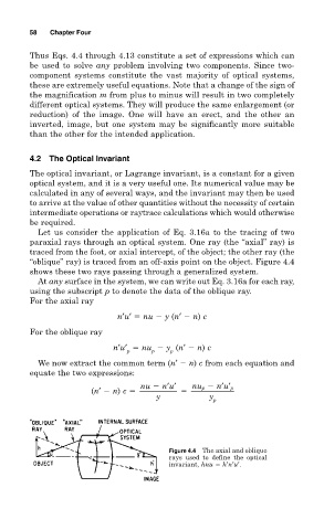
Let us consider the application of Eq. 3.16a to the tracing of two
paraxial rays through an optical system. One ray (the “axial” ray) is
traced from the foot, or axial intercept, of the object; the other ray (the
“oblique” ray) is traced from an off-axis point on the object. Figure 4.4
shows these two rays passing through a generalized system.
At any surface in the system, we can write out Eq. 3.16a for each ray,
using the subscript p to denote the data of the oblique ray.
For the axial ray
n′u′ nu y (n′ n) c
For the oblique ray

n′u′ nu y (n′ n) c
p p p
We now extract the common term (n′ n) c from each equation and
equate the two expressions:
nu n′u′ nu p n′u′ p
(n′ n) c
y y p

Figure 4.4 The axial and oblique
rays used to define the optical
invariant, hnu h′n′u′.