Page 247 - Modern Spatiotemporal Geostatistics

228 Modern Spatiotemporal Geostatistics — Chapter 11

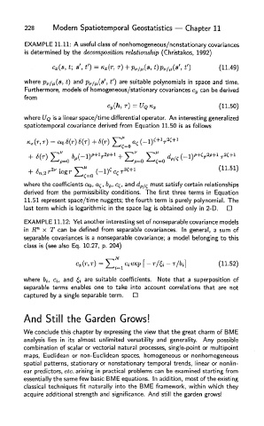
EXAMPLE 11.11: A useful class of nonhomogeneous/nonstationary covariances
is determined by the decomposition relationship (Christakos, 1992)

where p^/^s, t) and p^/p.(s', t') are suitable polynomials in space and time.
Furthermore, models of homogeneous/stationary covariances c y can be derived
from

where UQ is a linear space/time differential operator. An interesting generalized
spatiotemporal covariance derived from Equation 11.50 is as follows

where the coefficients a 0, a^, b p, c^, and dp/^ must satisfy certain relationships
derived from the permissibility conditions. The first three terms in Equation
11.51 represent space/time nuggets; the fourth term is purely polynomial. The
last term which is logarithmic in the space lag is obtained only in 2-D.

EXAMPLE 11.12: Yet another interesting set of nonseparable covariance models
in R n x T can be defined from separable covariances. In general, a sum of
separable covariances is a nonseparable covariance; a model belonging to this
class is (see also Eq. 10.27, p. 204)

where 6j, c it and & are suitable coefficients. Note that a superposition of
separable terms enables one to take into account correlations that are not
captured by a single separable term.

And Still the Garden Grows!

We conclude this chapter by expressing the view that the great charm of BME
analysis lies in its almost unlimited versatility and generality. Any possible
combination of scalar or vectorial natural processes, single-point or multipoint
maps, Euclidean or non-Euclidean spaces, homogeneous or nonhomogeneous
spatial patterns, stationary or nonstationary temporal trends, linear or nonlin-
ear predictors, etc. arising in practical problems can be examined starting from
essentially the same few basic BME equations. In addition, most of the existing
classical techniques fit naturally into the BME framework, within which they
acquire additional strength and significance. And still the garden grows!