Page 109 - Neural Network Modeling and Identification of Dynamical Systems

98 3. NEURAL NETWORK BLACK BOX APPROACH TO THE MODELING AND CONTROL OF DYNAMICAL SYSTEMS

methods can be proposed that take advantage influences the input–output model structure
of the specifics of these models to reduce the and its training procedure. Now we consider
computational complexity of the conventional the state space representation of a dynamical
methods for dynamic networks learning. Possi- system, which in the case of nonlinear system
ble ways of constructing such methods are dis- modeling, as noted above, is more general than
cussed in Chapters 2 and 5. the input–output representation [12–14].
Due to the nature of the impact of noise on the Let us first consider the case when noise af-
operation of parallel models, they can be used fects the output of the dynamical system. We
not only as one-step-ahead predictors, as is the assume that the required representation of the
case for serial-parallel models, but also as full- dynamical system has the following form:
fledged dynamical system models that allow us
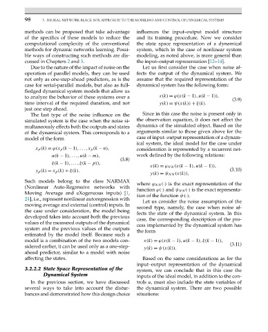
to analyze the behavior of these systems over a x(k) = ϕ(x(k − 1),u(k − 1)), (3.9)
time interval of the required duration, and not y(k) = ψ(x(k)) + ξ(k).
just one step ahead.
The last type of the noise influence on the Since in this case the noise is present only in
simulated system is the case when the noise si- the observation equation, it does not affect the
multaneously effects both the outputs and states dynamics of the simulated object. Based on the
of the dynamical system. This corresponds to a arguments similar to those given above for the
model of the form case of input–output representation of a dynam-
ical system, the ideal model for the case under
x p (k) = ϕ(x p (k − 1),...,x p (k − n), consideration is represented by a recurrent net-
u(k − 1),...,u(k − m), work defined by the following relations:
(3.8)
ξ(k − 1),...,ξ(k − p)),
x(k) = ϕ NN (x(k − 1),u(k − 1)),
y p (k) = x p (k) + ξ(k). (3.10)
y(k) = ψ NN (x(k)),
Such models belong to the class NARMAX where ϕ NN (·) is the exact representation of the
(Nonlinear Auto-Regressive networks with function ϕ(·) and ψ NN (·) is the exact representa-
Moving Average and eXogeneous inputs) [1,
tion of the function ψ(·).
24], i.e., represent nonlinear autoregression with
Let us consider the noise assumption of the
moving average and external (control) inputs. In
second type, namely, the case when noise af-
the case under consideration, the model being
fects the state of the dynamical system. In this
developed takes into account both the previous case, the corresponding description of the pro-
values of the measured outputs of the dynamical cess implemented by the dynamical system has
system and the previous values of the outputs the form
estimated by the model itself. Because such a
model is a combination of the two models con- x(k) = ϕ(x(k − 1),u(k − 1),ξ(k − 1)),
sidered earlier, it can be used only as a one-step- y(k) = ψ(x(k)). (3.11)
ahead predictor, similar to a model with noise
affecting the states. Based on the same considerations as for the
input–output representation of the dynamical
3.2.2.2 State Space Representation of the system, we can conclude that in this case the
Dynamical System inputs of the ideal model, in addition to the con-
In the previous section, we have discussed trols u, must also include the state variables of
several ways to take into account the distur- the dynamical system. There are two possible
bances and demonstrated how this design choice situations: