Page 151 - Neural Network Modeling and Identification of Dynamical Systems

4.3 APPLICATION OF ANN MODELS TO ADAPTIVE CONTROL PROBLEMS UNDER UNCERTAINTY CONDITIONS 141

u
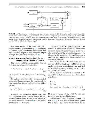
FIGURE 4.6 The neural network–based model reference adaptive control (MRAC) scheme. Here is control signal at the
output of the neurocontroller, u add is additional control from the compensator, u is resulting control, y p is output of the
y
controlled object (plant), is output of the neural network model of the plant; y rm is output of the reference model; ε is the
difference between the outputs of the plant and the reference model; ε m is the difference between the outputs of the plant
and the ANN model; r is the reference signal.

The ANN model of the controlled object, The use of the MRAC scheme requires to de-
whose structure is shown in Fig. 4.2,isfed with termine in one way or another the appropriate
the control signal from the neurocontroller, and reference model reflecting the developer’s views
also with the output of the controlled object of what the “good” behavior of this system looks
through the time delay lines. See Fig. 4.7. like so that the neurocontroller would attempt to
make the controlled system follow this behavior
4.3.2.2 Neurocontroller Synthesis for the
Model Reference Adaptive Control as close as possible.
We can define the reference model in vari-
The equation of the neurocontroller has the
following form (for static controllers): ous ways. In this chapter, we build the reference
model combining an oscillating-type unit with
u k = f(r k ,r k−1 ,...,r k−d ,y k ,y k−1 ,...,y k−d ), sufficiently high damping in combination with
an aperiodic-type unit.
(4.4)
In the case the motion of an aircraft is de-
where y is the plant output, r is the reference sig- scribed by (4.2), the reference model is defined
nal. as follows:
By analogy with the model reference control
scheme for linear systems, the equation of the ˙ x 1 = x 2 ,
neurocontroller should look somewhat differ-
˙ x 2 = x 3 ,
ent, i.e.,
˙ x 3 = ω act (−x 3 − 2ω rm ζ rm x 2 + ω 2 (r − x 1 )).
rm
u k = f(r k ,u k−1 ,...,u k−d ,y k ,y k−1 ,...,y k−d ). (4.6)
(4.5)
However, the simulation shows that these Here ω act = 40, ω rm = 3, ζ rm = 0.8. The state vec-
two implementations provide similar results, tor is x =[α rm , ˙α rm ,ϕ act ] in this case.
but the former learns a little faster. Therefore, Another version of the reference model, sim-
we adopt the static version (4.4) of the neuro- ilar to (4.6), is also a third-order linear system
controller as the main one. that is defined by a transfer function of the fol-