Page 126 - Numerical Analysis Using MATLAB and Excel

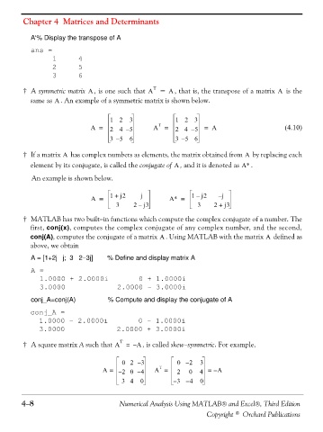
Chapter 4 Matrices and Determinants

A'% Display the transpose of A
ans =
1 4
2 5
3 6
T
†A symmetric matrix , is one such that A = , that is, the transpose of a matrix is the
A
A
A
same as . An example of a symmetric matrix is shown below.
A
12 3 12 3
T
A = 24 – 5 A = 24 – 5 = A (4.10)
–
35 6 35 6
–
† If a matrix has complex numbers as elements, the matrix obtained from by replacing each
A
A
element by its conjugate, is called the conjugate of , and it is denoted as A∗ .
A
An example is shown below.

A = 1 + j2 j A∗ = 1 – j2 j –
–
3 2 j3 3 2 + j3
† MATLAB has two built−in functions which compute the complex conjugate of a number. The
first, conj(x), computes the complex conjugate of any complex number, and the second,
conj(A), computes the conjugate of a matrix . Using MATLAB with the matrix defined as
A
A
above, we obtain

A = [1+2j j; 3 2−3j] % Define and display matrix A
A =
1.0000 + 2.0000i 0 + 1.0000i
3.0000 2.0000 - 3.0000i
conj_A=conj(A) % Compute and display the conjugate of A

conj_A =
1.0000 - 2.0000i 0 - 1.0000i
3.0000 2.0000 + 3.0000i
T
†A square matrix A such that A = – A , is called skew−symmetric. For example,

02 – 3 0 – 2 3
T
A = – 2 0 – 4 A = 2 0 4 = – A
34 0 – 3 – 4 0

4−8 Numerical Analysis Using MATLAB® and Excel®, Third Edition

Copyright © Orchard Publications