Page 280 - Numerical Analysis and Modelling in Geomechanics

ENRICO PRIOLO 261

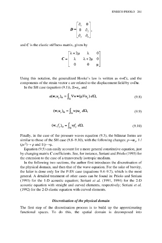
and C is the elastic stiffness matrix, given by

Using this notation, the generalized Hooke’s law is written as σ=Cε, and the
components of the strain vector ε are related to the displacement field by ε=Du.
In the SH case (equation (9.1)), Ξ=u , and
y
(9.8)

(9.9)

(9.10)

Finally, in the case of the pressure waves equation (9.3), the bilinear forms are
similar to those of the SH case (9.8–9.10), with the following changes: p→u , 1 /
y
2
(ρc )→ ρ and 1/ρ→µ.
Equation (9.5) can easily account for a more general constitutive equation, just
by changing matrix C coefficients. See, for instance, Seriani and Priolo (1995) for
the extension to the case of a transversely isotropic medium.
In the following two sections, the author first introduces the discretisation of
the physical domain, and then that of the wave equation. For the sake of brevity,
the latter is done only for the P-SV case (equations 9.4–9.7), which is the most
general. A detailed treatment of other cases can be found in: Priolo and Seriani
(1991) for the 1-D acoustic equation; Seriani et al. (1991, 1994) for the 2-D
acoustic equation with straight and curved elements, respectively; Seriani et al.
(1992) for the 2-D elastic equation with curved elements.

Discretisation of the physical domain

The first step of the discretisation process is to build up the approximating
functional spaces. To do this, the spatial domain is decomposed into