Page 123 - Numerical Methods for Chemical Engineering

112 3 Matrix eigenvalue analysis

Im(λ)

λ = a + ib

b
Γ
Γ 1 2
a 11 a a 22 Re(λ)

Γ = a 12 + a 13 + ... + a 1N
1
Γ = a 21 + a 23 + a 24 + ... + a 2N
2

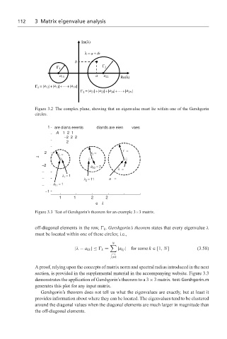
Figure 3.2 The complex plane, showing that an eigenvalue must lie within one of the Gershgorin
circles.

1 are diana eeents diands are eien vaes
A 1 2 1
−2 2 2
2
r =
2 r = r =
2
λ 1
−2 a = 2
22 λ =
−
= 1
− a =
λ 1
λ 2 = 11
− a 11 = 1
−1
1 1 2 2
e λ
Figure 3.3 Test of Gershgorin’s theorem for an example 3×3 matrix.

off-diagonal elements in the row, k . Gershgorin’s theorem states that every eigenvalue λ
must be located within one of these circles; i.e.,
N

|λ − a kk |≤ k = |a kj | for some k ∈ [1, N] (3.58)
j=1
j =k
A proof, relying upon the concepts of matrix norm and spectral radius introduced in the next
section, is provided in the supplemental material in the accompanying website. Figure 3.3
demonstrates the application of Gershgorin’s theorem to a 3 × 3 matrix. test-Gershgorin.m
generates this plot for any input matrix.
Gershgorin’s theorem does not tell us what the eigenvalues are exactly, but at least it
provides information about where they can be located. The eigenvalues tend to be clustered
around the diagonal values when the diagonal elements are much larger in magnitude than
the off-diagonal elements.