Page 41 - Numerical Methods for Chemical Engineering

30 1 Linear algebra

A
ℜ ℜ
A
w 0
A 0
Av ≠ 0
v
A
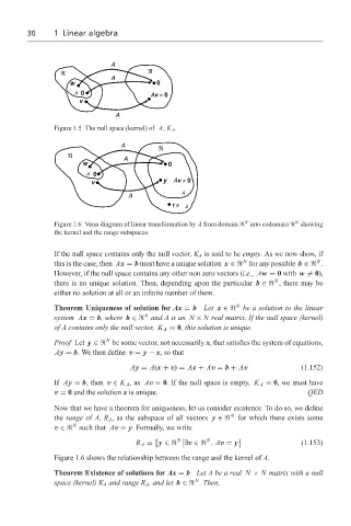
Figure 1.5 The null space (kernel) of A, K A .

A ℜ
ℜ
A
w 0
A 0
v y Av ≠ 0
A
A
r ∉ A

N
N
Figure 1.6 Venn diagram of linear transformation by A from domain into codomain showing
the kernel and the range subspaces.
If the null space contains only the null vector, K A is said to be empty.Aswenowshow,if
N
N
this is the case, then Ax = b must have a unique solution x ∈ for any possible b ∈ .
However, if the null space contains any other non zero vectors (i.e., Aw = 0 with w = 0),
N
there is no unique solution. Then, depending upon the particular b ∈ , there may be
either no solution at all or an infinite number of them.
N
Theorem Uniqueness of solution for Ax = b Let x ∈ be a solution to the linear
N
system Ax = b, where b ∈ andAisan N × N real matrix. If the null space (kernel)
of A contains only the null vector, K A = 0, this solution is unique.
N
Proof Let y ∈ be some vector, not necessarily x, that satisfies the system of equations,
Ay = b. We then define v = y − x, so that
Ay = A(x + v) = Ax + Av = b + Av (1.152)

If Ay = b, then v ∈ K A ,as Av = 0. If the null space is empty, K A = 0, we must have
v = 0 and the solution x is unique. QED
Now that we have a theorem for uniqueness, let us consider existence. To do so, we define
N
the range of A, R A , as the subspace of all vectors y ∈ for which there exists some
N
v ∈ such that Av = y. Formally, we write
N
R A ≡ y ∈ ∃v ∈ , Av = y (1.153)
N
Figure 1.6 shows the relationship between the range and the kernel of A.
Theorem Existence of solutions for Ax = b LetAbeareal N × N matrix with a null
N
space (kernel) K A and range R A , and let b ∈ . Then,