Page 85 - Numerical Methods for Chemical Engineering

74 2 Nonlinear algebraic systems

1
at west int 2 s is a stin

2

2

1

2 2
1 2

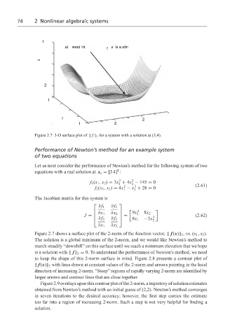
Figure 2.7 3-D surface plot of f 2 for a system with a solution at (3,4).

Performance of Newton’s method for an example system
of two equations

Let us next consider the performance of Newton’s method for the following system of two
T
equations with a real solution at x s = [3 4] :
3
2
f 1 (x 1 , x 2 ) = 3x + 4x − 145 = 0
2
1
3
2
f 2 (x 1 , x 2 ) = 4x − x + 28 = 0 (2.61)
2
1
The Jacobian matrix for this system is
 
∂ f 1 ∂ f 1
2
∂x 1 1
  9x 8x 2
J =  ∂x 2  = 2 (2.62)
 ∂ f 2 ∂ f 2  8x 1 −3x 2
∂x 1 ∂x 2
Figure 2.7 shows a surface plot of the 2-norm of the function vector, f (x) 2 , vs. (x 1 , x 2 ).
The solution is a global minimum of the 2-norm, and we would like Newton’s method to
march steadily “downhill” on this surface until we reach a minimum elevation that we hope
is a solution with f 2 = 0. To understand the performance of Newton’s method, we need
to keep the shape of this 2-norm surface in mind. Figure 2.8 presents a contour plot of
f (x) 2 with lines drawn at constant values of the 2-norm and arrows pointing in the local
direction of increasing 2-norm. “Steep” regions of rapidly varying 2-norm are identified by
larger arrows and contour lines that are close together.
Figure 2.9 overlays upon this contour plot of the 2-norm, a trajectory of solution estimates
obtained from Newton’s method with an initial guess of (2,2). Newton’s method converges
in seven iterations to the desired accuracy; however, the first step carries the estimate
too far into a region of increasing 2-norm. Such a step is not very helpful for finding a
solution.