Page 113 -

96 3. Finite Element Methods for Linear Elliptic Problems

The above question can therefore be reformulated as follows: Is it possible
2
to interpret v on ∂Ω as a function of L (∂Ω) (∂Ω“⊂” R d−1 )?
It is indeed possible if we have some minimal regularity of ∂Ωin the
following sense: It has to be possible to choose locally, for some boundary
point x ∈ ∂Ω, a coordinate system in such a way that the boundary is
locally a hyperplane in this coordinate system and the domain lies on one
side. Depending on the smoothness of the parametrisation of the hyperplane
k
we then speak of Lipschitz, C -(for k ∈ N), and C - domains (for an exact
∞
definition see Appendix A.5).
Examples:

(1) A circle Ω = x ∈ R d
|x − x 0 | <R is a C -domain for all k ∈ N,
k
and hence a C -domain.
∞

(2) A rectangle Ω = x ∈ R d
0 <x i <a i ,i =1,... ,d is a Lipschitz
1
domain, but not a C -domain.

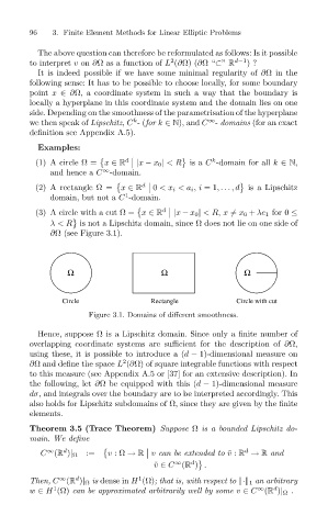
(3) A circle with a cut Ω = x ∈ R d
|x − x 0 | <R, x = x 0 + λe 1 for 0 ≤

λ< R is not a Lipschitz domain, since Ω does not lie on one side of
∂Ω (seeFigure3.1).

Ω Ω Ω

Circle Rectangle Circle with cut
Figure 3.1. Domains of different smoothness.

Hence, suppose Ω is a Lipschitz domain. Since only a finite number of
overlapping coordinate systems are sufficient for the description of ∂Ω,
using these, it is possible to introduce a (d − 1)-dimensional measure on
2
∂Ω and define the space L (∂Ω) of square integrable functions with respect
to this measure (see Appendix A.5 or [37] for an extensive description). In
the following, let ∂Ω be equipped with this (d − 1)-dimensional measure
dσ, and integrals over the boundary are to be interpreted accordingly. This
also holds for Lipschitz subdomains of Ω, since they are given by the finite
elements.
Theorem 3.5 (Trace Theorem) Suppose Ω is a bounded Lipschitz do-
main. We define

∞ d
d
C (R )| Ω := v :Ω → R v can be extended to ˜v : R → R and

d
∞
˜ v ∈ C (R ) .
1
d
Then, C (R )| Ω is dense in H (Ω);that is,withrespect to · 1 an arbitrary
∞
d
1
∞
w ∈ H (Ω) can be approximated arbitrarily well by some v ∈ C (R )| Ω .