Page 282 -

6.2. Finite Volume Method on Triangular Grids 265
.
a
i 2
Ω i 2 ,K
a
. S Ω . a
Ω i 3 ,K i 1 ,K i 1
.
a
i 3
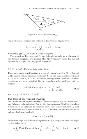
Figure 6.8. The subdomains Ω i k ,K .

required control volumes are defined as follows (see Figure 6.8):

#
Ω i := int Ω i,K , i ∈ Λ .
K:∂K
a i
The family {Ω i } is called a Donald diagram.
i∈Λ
The quantities Γ ij ,m ij , and Λ i are defined similarly as in the case of
the Voronoi diagram. We mention that the boundary pieces Γ ij are not
necessarily straight, but polygonal in general.

6.2.2 Finite Volume Discretization
The model under consideration is a special case of equation (6.1). Instead
of the matrix-valued diffusion coefficient K we will take a scalar coefficient
k :Ω → R, that is, K = kI. Moreover, homogeneous Dirichlet boundary
conditions are to be satisfied. So the boundary value problem reads as
follows:
−∇ · (k ∇u − cu)+ ru = f in Ω ,
(6.5)
u =0 on ∂Ω ,
2
with k, r, f :Ω → R,c :Ω → R .
The Case of the Voronoi Diagram
Let the domain Ω be partioned by a Voronoi diagram and the correspond-
ing Delaunay triangulation. Due to the homogeneous Dirichlet boundary
conditions, it is sufficient to consider only those control volumes Ω i that
are associated with inner nodes a i ∈ Ω. Therefore, we denote the set of
indices of all inner nodes by

Λ:= i ∈ Λ a i ∈ Ω .

In the first step, the differential equation (6.5) is integrated over the single
control volumes Ω i :

− ∇· (k ∇u − cu) dx + ru dx = fdx , i ∈ Λ . (6.6)
Ω i Ω i Ω i