Page 34 -

0.5. Boundary and Initial Value Problems 17

source terms f 1 and f 2 and otherwise identical coefficient functions. Then
u 1 + γu 2 is a solution of the same differential equation with the source
term f 1 + γf 2 for arbitrary γ ∈ R. The same holds for linear boundary
conditions. The term solution of an (initial-) boundary value problem is
used here in a classical sense, yet to be specified, where all the quantities
occurring should satisfy pointwise certain regularity conditions (see Defini-
tion 1.1 for the Poisson equation). However, for variational solutions (see
Definition 2.2), which are appropriate in the framework of finite element
methods, the above statements are also valid.
Linear differential equations of second order in two variables (x, y)(in-
cluding possibly the time variable) can be classified in different types as
follows:
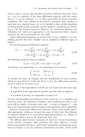
To the homogeneous differential equation

∂ 2 ∂ 2 ∂ 2
Lu = a(x, y) u + b(x, y) u + c(x, y) u
∂x 2 ∂x∂y ∂y 2 (0.44)
∂ ∂
+ d(x, y) u + e(x, y) u + f(x, y)u =0
∂x ∂y
the following quadratic form is assigned:
2
2
(ξ, η) → a(x, y)ξ + b(x, y)ξη + c(x, y)η . (0.45)
According to its eigenvalues, i.e., the eigenvalues of the matrix

1
a(x, y) b(x, y)
2 , (0.46)
1 b(x, y) c(x, y)
2
we classify the types. In analogy with the classification of conic sections,
which are described by (0.45) (for fixed (x, y)), the differential equation
(0.44) is called at the point (x, y)
• elliptic if the eigenvalues of (0.46) are not 0 and have the same sign,
• hyperbolic if one eigenvalue is positive and the other is negative,

• parabolic if exactly one eigenvalue is equal to 0.
For the corresponding generalization of the terms for d +1 variables and
arbitrary order, the stationary boundary value problems we treat in this
book will be elliptic, of second order, and — except in Chapter 8 — also
linear; the nonstationary initial-boundary value problems will be parabolic.
Systems of hyperbolic differential equations of first order require partic-
ular approaches, which are beyond the scope of this book. Nevertheless,
we dedicate Chapter 9 to convection-dominated problems, i.e., elliptic or
parabolic problems close to the hyperbolic limit case.
The different discretization strategies are based on various formulations
of the (initial-) boundary value problems: The finite difference method,
which is presented in Section 1, and further outlined for nonstationary prob-
lems in Chapter 7, has the pointwise formulation of (0.33), (0.36)–(0.38)