Page 203 - Numerical methods for chemical engineering

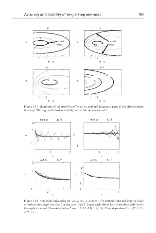
Accuracy and stability of single-step methods 189

θ θ

2
ω 1 staiit ω staiit
ndar 2 ndar
2

1 2 1 2
e ω e ω
θ θ 1

2
2
ω ω

2
1 2 1 2
e ω e ω

Figure 4.11 Magnitude of the growth coefficient vs. real and imaginary parts of the dimensionless
time step. The region of absolute stability lies within the contour of 1.

eicit er ∆t 2 eicit er ∆t 2
2
1
t t

1
1
1 2 1 2
t t
iicit er ∆t 2 iicit er ∆t 2
2
2
1
1
t t
1

1 2
2 1
t t
Figure 4.12 Numerical trajectories for dx/dt =−x, x(0) = 1 for explicit Euler and implicit Euler
at various time steps less than 2 and greater than 2. Upper right shows loss of absolute stability for
the explicit method. Time steps below 2 are {0.1, 0.5, 1.0, 1.5, 1.9}. Time steps above 2 are {2.1, 2.5,
2.75, 3}.