Page 217 - Numerical methods for chemical engineering

Parametric continuation 203

X Θ 1
s
X Θλ s
s

X s
X Θ rnin
s
ints
s
λ λ λ 1

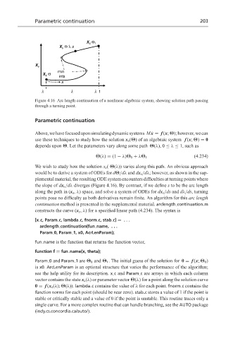
Figure 4.16 Arc length continuation of a nonlinear algebraic system, showing solution path passing
through a turning point.

Parametric continuation

Above,wehavefocuseduponsimulatingdynamicsystems M ˙ x = f (x; Θ);however,wecan
use these techniques to study how the solution x s (Θ) of an algebraic system f (x; Θ) = 0
depends upon Θ. Let the parameters vary along some path Θ(λ), 0 ≤ λ ≤ 1, such as

(4.234)
Θ(λ) = (1 − λ)Θ 0 + λΘ 1
We wish to study how the solution x s ( Θ(λ)) varies along this path. An obvious approach
would be to derive a system of ODEs for dΘ/dλ and dx s /dλ; however, as shown in the sup-
plemental material, the resulting ODE system encounters difficulties at turning points where
the slope of dx s /dλ diverges (Figure 4.16). By contrast, if we define s to be the arc length
along the path in (x s , λ) space, and solve a system of ODEs for dx s /ds and dλ/ds, turning
points pose no difficulty as both derivatives remain finite. An algorithm for this arc length
continuation method is presented in the supplemental material. arclength continuation.m
constructs the curve (x s , λ) for a specified linear path (4.234). The syntax is
[x c, Param c, lambda c, fnorm c, stab c] = ...
arclength continuation(fun name, . . .
Param 0, Param 1, x0, AcrLenParam);
fun name is the function that returns the function vector,
function f = fun name(x, theta);

Param 0 and Param 1 are Θ 0 and Θ 1 . The initial guess of the solution for 0 = f (x; Θ 0 )
is x0. ArcLenParam is an optional structure that varies the performance of the algorithm;
see the help utility for its description. x c and Param c are arrays in which each column
vector contains the state x s (λ) or parameter vector Θ(λ) for a point along the solution curve
0 = f (x s (λ); Θ(λ)). lambda c contains the value of λ for each point. fnorm c contains the
function norms for each point (should be near zero). stab c stores a value of 1 if the point is
stable or critically stable and a value of 0 if the point is unstable. This routine traces only a
single curve. For a more complex routine that can handle branching, see the AUTO package
(indy.cs.concordia.ca/auto/).