Page 19 - PRINCIPLES OF QUANTUM MECHANICS as Applied to Chemistry and Chemical Physics

10 The wave function

narrow and ù(k) changes slowly with k, so that the variation in v g is small.
Combining equations (1.15) and (1.16), we have
1 1
B(x, t) ˆ p  A(k)e i(xÿv g t)(kÿk 0 ) dk (1:17)
2ð ÿ1
Since the function A(k) is the Fourier transform of Ø(x, t), the two functions
obey Parseval's theorem as given by equation (B.28) in Appendix B

1 1 1
2 2 2
jØ(x, t)j dx ˆ jB(x, t)j dx ˆ jA(k)j dk (1:18)
ÿ1 ÿ1 ÿ1

Gaussian wave number distribution
In order to obtain a speci®c mathematical expression for the wave packet, we
need to select some form for the function A(k). In our ®rst example we choose
A(k) to be the gaussian function
1 ÿ(kÿk 0 ) =2á 2
2
A(k) ˆ p  e (1:19)
2ðá
This function A(k) is a maximum at wave number k 0 , which is also the average
value for k for this distribution of wave numbers. Substitution of equation
(1.19) into (1.17) gives
1 ÿá (xÿv g t) =2
2
2
jØ(x, t)jˆ B(x, t) ˆ p  e (1:20)
2ð
where equation (A.8) has been used. The resulting modulating factor B(x, t)is
also a gaussian function±following the general result that the Fourier transform
of a gaussian function is itself gaussian. We have also noted in equation (1.20)
that B(x, t) is always positive and is therefore equal to the absolute value
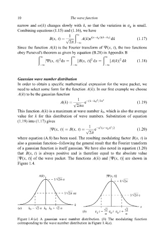
jØ(x, t)j of the wave packet. The functions A(k) and jØ(x, t)j are shown in
Figure 1.4.

A(k) |Ψ(x, t)|
1/Ö2π α
1/Ö2π

1/Ö2π αe
1/Ö2π e

k
(a) k 2 Ö2 α k 0 k 1 Ö2 α Ö2 Ö2 x
0
0
(b) v g t 2 v t v t 1
g
g
α α
Figure 1.4 (a) A gaussian wave number distribution. (b) The modulating function
corresponding to the wave number distribution in Figure 1.4(a).