Page 181 -

5.4 Neural Network Types 169

For instance, a two-class six-dimensional problem solved by an MLP6:4:2
involves the computation of 38 weights. The number of these weights, which are
the parameters of the neural net, measures its complexity. Imagine that we had
succeeded in designing an optimal Bayesian linear discriminant for the same two-
class six-dimensional problem. The statistical classifier solution demands the
computation of two six-dimensional mean vectors plus d(d+1)/2=21 elements of
the covariance matrix, totalling 33 parameters. Even if the neural net would
perfectly mimic the statistical classifier, it represents a more complex and
expensive classifier, with more parameters to adjust. Complex classifiers are harder
to train adequately and need larger training sets for proper generalization.
Whenever possible, a model-based statistical classifier turns out to be simpler than
an equivalently performing neural network. Of course, a model-based statistical
approach is not always feasible, and the neural network approach is then a sensible
choice.

. . . .

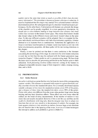
delay units
Figure 5.22. A Hopfield network structure with feedback through delay elements.

The MLP network is a feed-forward structure, whose only paths are from the
inputs to the outputs. It is also possible to have neural net architectures
(connectionist structures) with feedback paths, connecting outputs to inputs of
previous layers through delay elements and without self-feedback, i.e., no neuron
output is fed back to its own input. Figure 5.22 shows a Hopjield network, an
example of such architectures, also called recurrent networks, which exhibit non-
linear dynamical behaviour with memory properties.
All these types of neural nets are trained in a supervised manner, using the
pattern classification information of a training set. There are also unsupervised
types of neural networks, such as the Kohonen's self organising feature map
(KFM) that we will present in section 5.1 1.