Page 237 -

5.1 1 Kohonen Networks 225

Neurons outside the neighbourhood are not updated. Also, the neighbourhood
does not wrap around the borders.
4 Update learning rate and neighbourhood radius (decreasing them).
5. Repeat steps 2 to 4 until the stopping condition (e.g. maximum number of
epochs) is reached.

The Kohonen network develops a sort of two-dimensional map, resembling the
application of multidimensional scaling techniques. The effect of the
neighbourhood is to drag the training cases near their winning prototypes. As the
network training progresses, the decrease of neighbourhood radius and learning
rate will result in a finer tuning of each neuron to the most similar input pattern.
After a sufficient number of epochs the weights will cluster, such that the grid of
output neurons constitutes a kind of topological map of the inputs, reflecting the
structure of the data, therefore the name of self-organizing map. The performance
of the mapping is evaluated by an error measure that averages, for all patterns, the
distance dik of each pattern from the winning output neuron.

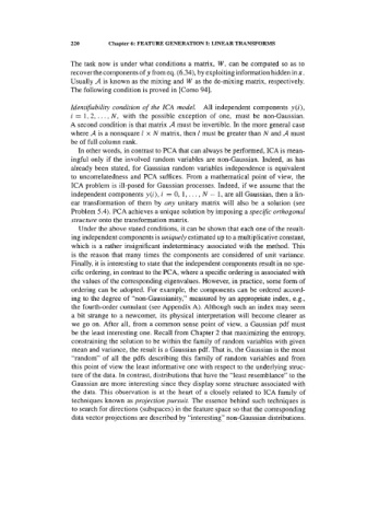
Table 5.8. Winning frequencies for a Kohonen network trained with the globular
data shown in Figure 3.4a.
(4 (b)

z2.
0

(a) 10 epochs with =O. 1, -2.
(b) Convergence situation with ~0.05, r=l

We now proceed to exemplify the use of a Kohonen mapping, using Statistica.
We start with the globular data of Cluster.xls shown in Figure 3.4a. We use a 3x3
output grid and start with a neighbourhood radius of 2. Training with only 10
epochs and a learning rate of 0.1 we obtain the winning frequencies, i.e., the
number of patterns for which an output neuron is a winning neuron, shown in
Table 5.8. The error (sum of dik) is then around 0.4. Looking at the local maxima it
seems that a cluster centre is forming around zz3 and possibly another one at zll.
With further training using a neighbourhood radius of 1 and a smaller learning rate,
we reach the solution shown in Table 5.8 with an error below 0.2, where it is
clearly visible that there are now two distinct clusters represented by (zll) and
(233, 223). separated by zero cases at 222 and only isolated borderline cases, e.g. at
231 and zl3.