Page 142 - Physical Chemistry

lev38627_ch04.qxd 2/29/08 3:13 PM Page 123

123
Section 4.5
6
6
From Sec. 8.4, a 1.35 10 cm atm mol 2 for N . At 25°C and 1 atm, the Calculation of Changes
2
gas is nearly ideal and V/n can be found from PV nRT with little error. We get in State Functions
3
3
V/n 24.5 10 cm /mol. Thus
2
6
6
3
3
10U>0V2 11.35 10 cm atm>mol 2>124.5 10 cm >mol2 2
T
3
3
10.0022 atm218.314 J2>182.06 cm atm2 0.00023 J>cm
0.23 J>L (4.58)
The smallness of (
U/
V) indicates the smallness of intermolecular forces in N 2
T
gas at 25°C and 1 atm.
Exercise
Use the van der Waals equation and data in Sec. 8.4 to estimate (
U/
V) for
T
HCl(g) at 25°C and 1 atm. Why is (
U/
V) larger for HCl(g) than for N (g)?
T
2
[Answer: 0.0061 atm 0.62 J/L.]
U intermol of a liquid can be estimated as U of vaporization.
4.5 CALCULATION OF CHANGES IN STATE FUNCTIONS
Section 2.9 discussed calculation of U and H in a process, and Sec. 3.4 discussed
calculation of S. These discussions were incomplete, since we did not have expres-
sions for (
U/
V) , for (
H/
P) , and for (
S/
P) in paragraph 8 of Sec. 3.4. We now
T
T
T
have expressions for these quantities. Knowing how U, H, and S vary with T, P, and V,
we can find U, H, and S for an arbitrary process in a closed system of constant
composition. We shall also consider calculation of A and G.
Calculation of S
Suppose a closed system of constant composition goes from state (P , T ) to state
1
1
(P , T ) by any path, including, possibly, an irreversible path. The system’s entropy is
2
2
a function of T and P; S S(T, P), and
0S 0S C P
dS a b dT a b dP dT aV dP (4.59)
0T P 0P T T
where (4.49) and (4.50) were used. Integration gives
1
¢S S S 2 C P dT 2 aV dP (4.60)
2
1 T 1
Since C , a, and V depend on both T and P, these are line integrals [unlike the integral
P
in the perfect-gas S equation (3.30)].
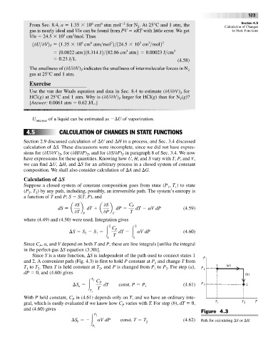
Since S is a state function, S is independent of the path used to connect states 1
and 2. A convenient path (Fig. 4.3) is first to hold P constant at P and change T from
1
T to T . Then T is held constant at T , and P is changed from P to P . For step (a),
1
1
2
2
2
dP 0, and (4.60) gives
a T 2 C P
¢S dT const. P P 1 (4.61)
T
T 1
With P held constant, C in (4.61) depends only on T, and we have an ordinary inte-
P
gral, which is easily evaluated if we know how C varies with T. For step (b), dT 0,
P
and (4.60) gives
Figure 4.3
P 2
¢S aV dP const. T T 2 (4.62) Path for calculating S or H.
b
P 1