Page 340 - Probability and Statistical Inference

6. Sufficiency, Completeness, and Ancillarity 317

Fisher (1934, 1956) in the famous “Nile” example. One may also refer to
Basu (1964), Hinkley (1980a), Ghosh (1988) and Reid (1995) for fuller dis-
cussions of conditional inference.
The approach goes through the following steps. One first finds the condi-
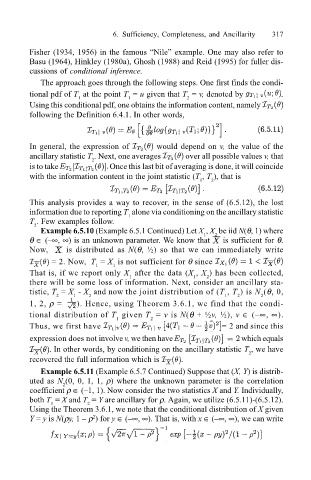
tional pdf of T at the point T = u given that T = v, denoted by .
2
1
1
Using this conditional pdf, one obtains the information content, namely
following the Definition 6.4.1. In other words,

In general, the expression of would depend on v, the value of the
ancillary statistic T . Next, one averages over all possible values v, that
2
is to take Once this last bit of averaging is done, it will coincide
with the information content in the joint statistic (T , T ), that is
1 2

This analysis provides a way to recover, in the sense of (6.5.12), the lost
information due to reporting T alone via conditioning on the ancillary statistic
1
T . Few examples follow.
2
Example 6.5.10 (Example 6.5.1 Continued) Let X , X be iid N(θ, 1) where
1
θ ∈ (–∞, ∞) is an unknown parameter. We know that 2 is sufficient for θ.
Now, is distributed as N(θ, ½) so that we can immediately write
= 2. Now, T = X is not sufficient for θ since
1 1
That is, if we report only X after the data (X , X ) has been collected,
1
2
1
there will be some loss of information. Next, consider an ancillary sta-
tistic, T = X - X and now the joint distribution of (T , T ) is N (θ, 0,
2 1 2 1 2 2
1, 2, ρ = ). Hence, using Theorem 3.6.1, we find that the condi-
tional distribution of T given T = v is N(θ + ½v, ½), v ∈ (–∞, ∞).
1 2
Thus, we first have = 2 and since this
expression does not involve v, we then have which equals
. In other words, by conditioning on the ancillary statistic T , we have
2
recovered the full information which is .
Example 6.5.11 (Example 6.5.7 Continued) Suppose that (X, Y) is distrib-
uted as N (0, 0, 1, 1, ρ) where the unknown parameter is the correlation
2
coefficient ρ ∈ (–1, 1). Now consider the two statistics X and Y. Individually,
both T = X and T = Y are ancillary for ρ. Again, we utilize (6.5.11)-(6.5.12).
2
1
Using the Theorem 3.6.1, we note that the conditional distribution of X given
Y = y is N(ρy, 1 – ρ ) for y ∈ (–∞, ∞). That is, with x ∈ (–∞, ∞), we can write
2