Page 600 - Probability and Statistical Inference

13. Sample Size Determination: Two-Stage Procedures 577

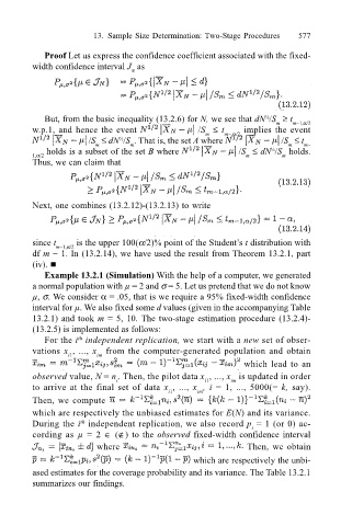
Proof Let us express the confidence coefficient associated with the fixed-
width confidence interval J as
N

But, from the basic inequality (13.2.6) for N, we see that dN /S ≥ t m−1,α/2
½
m
w.p.1, and hence the event /S ≤ t m−,α/2 implies the event
m
/S ≤ dN /S . That is, the set A where /S ≤ t
½
m m m m−
holds is a subset of the set B where /S ≤ dN /S holds.
½
1,α/2 m m
Thus, we can claim that
Next, one combines (13.2.12)-(13.2.13) to write

since t m−1,α/2 is the upper 100(α/2)% point of the Student’s t distribution with
df m − 1. In (13.2.14), we have used the result from Theorem 13.2.1, part
(iv). !
Example 13.2.1 (Simulation) With the help of a computer, we generated
a normal population with µ = 2 and σ = 5. Let us pretend that we do not know
µ, σ. We consider α = .05, that is we require a 95% fixed-width confidence
interval for µ. We also fixed some d values (given in the accompanying Table
13.2.1) and took m = 5, 10. The two-stage estimation procedure (13.2.4)-
(13.2.5) is implemented as follows:
For the i independent replication, we start with a new set of obser-
th
vations x , ..., x from the computer-generated population and obtain
i1 im
which lead to an
observed value, N = n . Then, the pilot data x , ..., x is updated in order
i1
im
i
to arrive at the final set of data x , ..., x , i = 1, ..., 5000(= k, say).
i1 ini
Then, we compute
which are respectively the unbiased estimates for E(N) and its variance.
During the i independent replication, we also record p = 1 (or 0) ac-
th
i
cording as µ = 2 ∈ (∉) to the observed fixed-width confidence interval
where Then, we obtain
which are respectively the unbi-
ased estimates for the coverage probability and its variance. The Table 13.2.1
summarizes our findings.