Page 250 - Radiochemistry and nuclear chemistry

234 Radiochemistry and Nuclear Chemistry

.lO III!11 IIIIIII
.09 ,,o~.~. ~..m ,~o,, ~ f ~~
.08 //
.07
.06
/
F'OV) .os
.04 / F
/ \
.03 k
.02 r
./ \
.01
,00
0 2 4 6 8 10 12 14 16 18 20 22 24 26 28 30 32 34 36 38 40
N
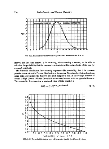
FIG. 8.23. Poisson (smooth) and Gaussian (dashed line) distributions for/9 = 20.

interval for the same sample. It is necessary, when counting a sample, to be able to
calculate the probability that the recorded count rate is within certain limits of the true (or
average) count rate.
The binomial distribution law correctly expresses this probability, but it is common
practice to use either the Poisson distribution or the normal Gaussian distribution functions
since both approximate the first but are much simpler to use. If the average number of
counts is high (above 100) the Gaussian function may be used with no appreciable error.
The probability for observing a measured value of total count N is

P(N) = (27r/9)- '~ e-"~(~'-~0~/tr (8.17)

2.6
2.4 ,~
2.2\
\
2.0
1.8 k .
\,.
1.6 \
~J.4 \
].2 %.
J.O
0.8
0.6
0.4
0.2
0.0
0.1 0.2 0.3 0.4 0.5 0.6 0.7 0.8 0.9 1.0
Probobility of error ) K
FIG. 8.24. The probability that an error will be greater than Ko for different K-values.