Page 353 - Schaum's Outline of Differential Equations

APPENDIX B

Some Comments

about Technology

INTRODUCTORY REMARKS
In this book we have presented many classical and time-honored methods to solve differential equations.
Virtually all these techniques produced closed-form analytical solutions. These solutions were of an exact
nature.
However, we have also discussed other approaches to differential equations; equations which did not easily
lend themselves to exact solutions. In Chapter 2, we touched upon the idea of qualitative approaches; Chapter 18
dealt with graphical methods; Chapters 19 and 20 investigated numerical techniques.
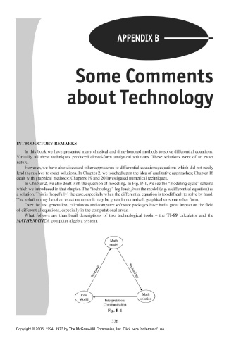
In Chapter 2, we also dealt with the question of modeling. In Fig. B-l, we see the "modeling cycle" schema
which we introduced in that chapter. The "technology" leg leads from the model (e.g. a differential equation) to
a solution. This is (hopefully) the case, especially when the differential equation is too difficult to solve by hand.
The solution may be of an exact nature or it may be given in numerical, graphical or some other form.
Over the last generation, calculators and computer software packages have had a great impact on the field
of differential equations, especially in the computational areas.
What follows are thumbnail descriptions of two technological tools - the TI-89 calculator and the
MATHEMATICA computer algebra system.

Fig. B-l

336
Copyright © 2006, 1994, 1973 by The McGraw-Hill Companies, Inc. Click here for terms of use.