Page 144 - Schaum's Outline of Theory and Problems of Signals and Systems

CHAP. 31 LAF'LACE TRANSFORM AND CONTINUOUS-TIME LTI SYSTEMS 133

Thus, combining the two results for a > 0 and a < 0, we can write these relationships as

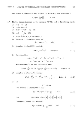
3.9. Find the Laplace transform and the associated ROC for each of the following signals:

(a) x(t) = S(t -to)
(b) x(t) = u(t - to)
(c) ~(t) e-"[u(t) - u(t - 5)]
=
ffi
(dl x(t) = S(t - kT)
k=O
(e) x(t) = S(at + b), a, b real constants

(a) Using Eqs. (3.13) and (3.161, we obtain
S(I - I,,) H e-s'fl all s

(b) Using Eqs. (3.14) and (3.16), we obtain

(c) Rewriting x(l) as

Then, from Table 3-1 and using Eq. (3.161, we obtain

(d) Using Eqs. (3.71) and (1.99), we obtain
m m 1
~(s) C e-.~'T= C (e-sT)li = Re(s) > 0 (3.73)
=
1 - esT
k=O k -0
(e) Let

f(0 = s(at)
Then from Eqs. (3.13) and (3.18) we have
1
f(t) = S(a1) - F(s) = - all s
la l

Now

Using Eqs. (3.16) and (3.741, we obtain
1
X(s) = esb/a~(S) -esh/" all s
=
la l