Page 273 - Schaum's Outline of Theory and Problems of Signals and Systems

FOURIER ANALYSIS OF TIME SIGNALS AND SYSTEMS [CHAP. 5

since a > 0. Thus, we get

dX(w) w
-- - - -X(w)
dw 2a
Solving the above separable differential equation for X(w), we obtain

where A is an arbitrary constant. To evaluate A we proceed as follows. Setting w = 0 in
Eq. (5.162) and by a change of variable, we have

Substituting this value of A into Eq. (5.1631, we get

Hence, we have

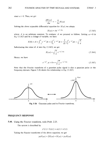
Note that the Fourier transform of a gaussian pulse signal is also a gaussian pulse in the
frequency domain. Figure 5-26 shows the relationship in Eq. (5.165).

Fig. 5-26 Gaussian pulse and its Fourier transform.

FREQUENCY RESPONSE

5.44. Using the Fourier transform, redo Prob. 2.25.

The system is described by
y'(t) + 2y(t) =x(t) +xf(t)
Taking the Fourier transforms of the above equation, we get
jwY(w) + 2Y(w) = X(w) +jwX(w)