Page 290 - Schaum's Outlines - Probability, Random Variables And Random Processes

CHAP. 91 QUEUEING THEORY

Assume that in the steady state we have

and setting pb(t) and pk(t) = 0 in Eqs. (9.6), we obtain the following steady-state recursive equation:
(an + dn)~n = an-lpn-1 + dn+lpn+l n 2 1
and for the special case with do = 0,

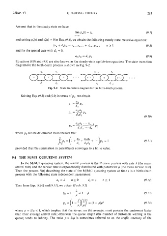
Equations (9.8) and (9.9) are also known as the steady-state equilibrium equations. The state transition
diagram for the birth-death process is shown in Fig. 9-2.

Fig. 9-2 State transition diagram for the birth-death process.

Solving Eqs. (9.8) and (9.9) in terms of p, , we obtain

where po can be determined from the fact that

provided that the summation in parentheses converges to a finite value.

9.4 THE M/M/1 QUEUEING SYSTEM

In the M/M/1 queueing system, the arrival process is the Poisson process with rate A (the mean
arrival rate) and the service time is exponentially distributed with parameter p (the mean service rate).
Then the process N(t) describing the state of the M/M/1 queueing system at time t is a birth-death
process with the Following state independent parameters:

Then from Eqs. (9.1 0) and (9.1 I), we obtain (Prob. 9.3)

where p = Alp < 1, which implies that the server, on the average, must process the customers faster
than their average arrival rate; otherwise the queue length (the number of customers waiting in the
queue) tends to infinity. The ratio p = Alp is sometimes referred to as the trafJic intensity of the