Page 220 - Semiconductor For Micro- and Nanotechnology An Introduction For Engineers

Local Equilibrium Description
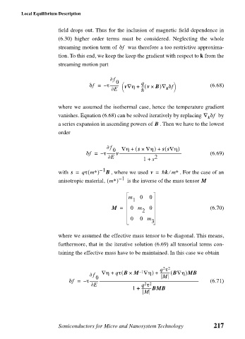
field drops out. Thus for the inclusion of magnetic field dependence in
(6.30) higher order terms must be considered. Neglecting the whole
streaming motion term of δf was therefore a too restrictive approxima-
tion. To this end, we keep the keep the gradient with respect to k from the
streaming motion part

f ∂
0
δf = – τ---------  v∇η + q B)∇ δf  (6.68)
--- v ×(
∂ E  — k 
where we assumed the isothermal case, hence the temperature gradient
vanishes. Equation (6.68) can be solved iteratively by replacing ∇ δf by
k
a series expansion in ascending powers of . Then we have to the lowest
B
order

f ∂ ∇η + ( s × ∇η) + ss∇η)
(
0
δf = – τ---------v------------------------------------------------------------------ (6.69)
∂ E 2
1 + s
(
⁄
with s = qτ m∗ ) – 1 B , where we used v = —k m∗ . For the case of an
(
anisotropic material, m∗ ) – 1 is the inverse of the mass tensor M
m 0 0
1
M = 0 m 0 (6.70)
2
0 0 m
3
where we assumed the effective mass tensor to be diagonal. This means,
furthermore, that in the iterative solution (6.69) all tensorial terms con-
taining the effective mass have to be maintained. In this case we obtain

2 2
q τ
–
1
f ∂ ∇η + qτ B ×( M ∇η) + ---------- B∇η( )MB
M
0
δf = – τ------------------------------------------------------------------------------------------------------------------ (6.71)
∂ E q τ
2 2
1 + ----------BMB
M
Semiconductors for Micro and Nanosystem Technology 217