Page 195 - Sensing, Intelligence, Motion : How Robots and Humans Move in an Unstructured World

170 ACCOUNTING FOR BODY DYNAMICS: THE JOGGER’S PROBLEM

u 2

q u 3 u 1 p

u 4 u 0
V i 8
u
C i
u 5
u 7

y u 6

S x

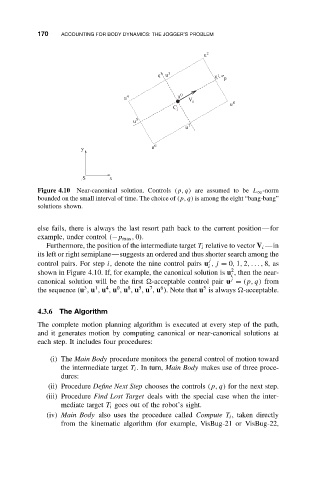
Figure 4.10 Near-canonical solution. Controls (p, q) are assumed to be L ∞ -norm
bounded on the small interval of time. The choice of (p, q) is among the eight “bang-bang”
solutions shown.

else fails, there is always the last resort path back to the current position—for
example, under control (−p max , 0).
Furthermore, the position of the intermediate target T i relative to vector V i —in
its left or right semiplane—suggests an ordered and thus shorter search among the
j
control pairs. For step i, denote the nine control pairs u ,j = 0, 1, 2,..., 8, as
i
2
shown in Figure 4.10. If, for example, the canonical solution is u , then the near-
i
j
canonical solution will be the first -acceptable control pair u = (p, q) from
5
8
7
6
5
4
1
3
0
the sequence (u , u , u , u , u , u , u , u ). Note that u is always -acceptable.
4.3.6 The Algorithm
The complete motion planning algorithm is executed at every step of the path,
and it generates motion by computing canonical or near-canonical solutions at
each step. It includes four procedures:
(i) The Main Body procedure monitors the general control of motion toward
the intermediate target T i . In turn, Main Body makes use of three proce-
dures:
(ii) Procedure Define Next Step chooses the controls (p, q) for the next step.
(iii) Procedure Find Lost Target deals with the special case when the inter-
mediate target T i goes out of the robot’s sight.
(iv) Main Body also uses the procedure called Compute T i , taken directly
from the kinematic algorithm (for example, VisBug-21 or VisBug-22,