Page 78 - Sensing, Intelligence, Motion : How Robots and Humans Move in an Unstructured World

MOTION PLANNING WITH COMPLETE INFORMATION 53

If the robot’s orientation in space is maintained constant for the duration
of its motion, the computation of C-space is relatively easy. If, in addition, the
robot and obstacles are 2D polygons, then the grown obstacles are also polygons,
though not necessarily with the same number of edges as in the original polygons
(Figure 2.15b).
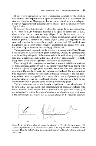
If, however, the robot orientation is allowed to change during the motion then,
the C-space for a 2D workspace becomes a 3D space of parameters (x,y,θ),
where θ is the robot orientation angle (Figure 2.16a). In this case, even the
original polygonal robot and/or obstacles produce nonpolygonal and, in general,
nonlinear grown 3D obstacles in C-space (Figure 2.16b). As complexity of the
robot and obstacles increases—for example, in cases with 3D multilink arm
manipulators and nonpolygonal obstacles—computation and proper representa-
tion of the C-space becomes an exceedingly difficult task.
The computational complexity of the problem is measured in the Piano Movers
model in terms of the connectivity graph’s structure. Overall, the computational
price for dealing with perfect information and for the said advantages—optimal
paths and, in principle, solutions for cases of arbitrary dimensionality—is high.
Today many reasonable-size problems still cannot be approached.
From the application standpoint, unless there is a reason to believe that obsta-
cle boundaries are algebraic (which would squarely mean that we are dealing with
man-made objects), an appropriate approximation of the robot workspace has to
be performed before the connectivity graph can be calculated. The approximation
itself necessarily depends on considerations that are secondary to the path plan-
ning problem. One may specify, for example, the accuracy of presenting actual
obstacles with polygons, or—a different criterion—one may put a limit on the
computational cost of processing the resulting connectivity graph.
The approximation process can introduce significant computational costs of
its own. John Reif has shown that approximation of nonlinear surfaces with
linear constraints itself requires time exponential in the prescribed accuracy of
approximation [14]. Also, the space of possible approximations is not continuous
in the approximation accuracy; that is, a slight change in the specified accuracy

y y
p
l p
A
q l q
p
p
x 2 x
(a) (b)
Figure 2.16 (a) When robot orientation is added to a 2D task, the (b) resulting 3D
C-space of parameters (x, y, θ) is nonlinear, even if the original robot and obstacles are
polygons. Here the “robot” A is a line segment of length l, and the obstacle is a horizontal
“table” line.