Page 146 - Separation process engineering

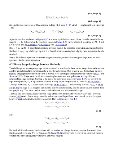
(4-6, stage k)

(4-7, stage k)

the equilibrium expression will correspond to Eqs. (4-4, stage f + 1) with k − 1 replacing f as a subscript.
Thus,

(4-4, stage k)

A partial reboiler as shown in Figure 4-2C acts as an equilibrium contact. If we consider the reboiler as
stage N + 1, the balances for the envelope shown in Figure 4-2C can be obtained by setting k = N + 1 and
k − 1 = N in Eqs. (4-5, stage k), (4-6, stage k) and (4-7, stage k).

If x N+1 = x , the N + 1 equilibrium contacts gives us exactly the specified separation, and the problem is
B
finished. If x < x while x > x , the N + 1 equilibrium contacts gives slightly more separation than is
N+1 B N B
required.
Just as the balance equations in the enriching section are symmetric from stage to stage, they are also
symmetric in the stripping section.

4.2 Binary Stage-by-Stage Solution Methods

The challenge for any stage-by-stage solution method is to solve the three balance equations and the three
equilibrium relationships simultaneously in an efficient manner. This problem was first solved by Sorel
(1893), and graphical solutions of Sorel’s method were developed independently by Ponchon (1921) and
Savarit (1922). These methods all solve the complete mass and energy balance and equilibrium
relationships stage by stage. Starting at the top of the column as shown in Figure 4-1A, we can find the
liquid composition, x , in equilibrium with the leaving vapor composition, y , from Eq. (4-4c, stage 1).
1
1
The liquid enthalpy, h , is easily found from Eqs. (4-4a, stage 1). The remaining four Eqs. (4-1) to (4-3)
1
and (4-4b) for stage 1 are coupled and must be solved simultaneously. The Ponchon-Savarit method does
this graphically. The Sorel method uses a trial-and-error procedure on each stage.

The trial-and-error calculations on every stage of the Sorel method are obviously slow and laborious.
Lewis (1922) noted that in many cases the molar vapor and liquid flow rates in each section (a region
between input and output ports) were constant. Thus in Figures 4-1 and 4-2,

(4-8)

and

(4-9)

For each additional column section there will be another set of equations for constant flow rates. Note
that in general L ≠ and V ≠ . Equations (4-8) and (4-9) will be valid if every time a mole of vapor is
condensed a mole of liquid is vaporized. This will occur if: