Page 251 -

234 5. Some worked examples arising from physical problems

Here, is the rate of molecular collisions (with the wall) between x and
and the rate contributed by those molecules that have their first collision
between these same stations. The kernel, K(x – y), measures the probability that a
molecule which has collided with the wall at x = y will collide again between the
stations. (This type of process is called a free-molecular or Knudsen flow.)
When we introduce the appropriate models for and non-
dimensionalise and use the symmetry of n(x) (i.e. n(x) + n(–x) = 0 so that n(0) = 0),
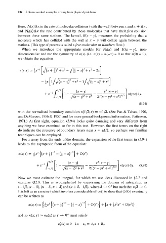
we obtain the equation

with the normalised boundary condition (See Pao & Tchao, 1970,
and DeMarcus, 1956 & 1957, and for more general background information, Patterson,
1971.) At first sight, equation (5.94) looks quite daunting and very different from
anything we have examined so far in this text. However, the first terms on the right
do indicate the presence of boundary layers near x = ±1/2, so perhaps our familiar
techniques can be employed.
For x away from the ends of the domain, the expansion of the first terms in (5.94)
leads to the asymptotic form of the equation:

Now we must estimate the integral, for which we use ideas discussed in §2.2 and
exercise Q2.8. This is accomplished by expressing the domain of integration as
and where but such that
It is left as an exercise (which involves considerable effort) to show that (5.95) eventually
can be written as

and so as must satisfy