Page 86 -

69

which the interested reader may wish to derive.) The two ‘expansions of expan-
sions’, (2.31) and (2.32), match when we choose and
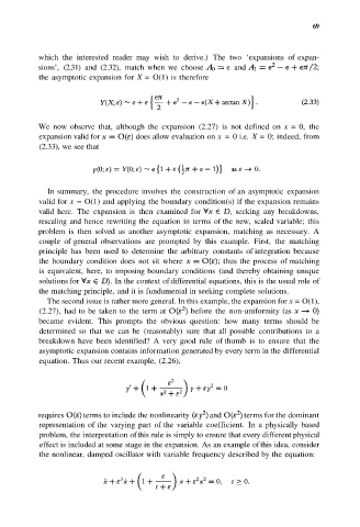
the asymptotic expansion for X = O(1) is therefore

We now observe that, although the expansion (2.27) is not defined on x = 0, the
expansion valid for does allow evaluation on x = 0 i.e. X = 0; indeed, from
(2.33), we see that

In summary, the procedure involves the construction of an asymptotic expansion
valid for x = O(1) and applying the boundary condition(s) if the expansion remains
valid here. The expansion is then examined for seeking any breakdowns,
rescaling and hence rewriting the equation in terms of the new, scaled variable; this
problem is then solved as another asymptotic expansion, matching as necessary. A
couple of general observations are prompted by this example. First, the matching
principle has been used to determine the arbitrary constants of integration because
the boundary condition does not sit where thus the process of matching
is equivalent, here, to imposing boundary conditions (and thereby obtaining unique
solutions for In the context of differential equations, this is the usual role of
the matching principle, and it is fundamental in seeking complete solutions.
The second issue is rather more general. In this example, the expansion for x = O(1),
(2.27), had to be taken to the term at before the non-uniformity (as
became evident. This prompts the obvious question: how many terms should be
determined so that we can be (reasonably) sure that all possible contributions to a
breakdown have been identified? A very good rule of thumb is to ensure that the
asymptotic expansion contains information generated by every term in the differential
equation. Thus our recent example, (2.26),

requires terms to include the nonlinearity and terms for the dominant
representation of the varying part of the variable coefficient. In a physically based
problem, the interpretation of this rule is simply to ensure that every different physical
effect is included at some stage in the expansion. As an example of this idea, consider
the nonlinear, damped oscillator with variable frequency described by the equation: