Page 316 -

Exercises 303

Exercises

(Section 6.1) pair-correlation function with Exerc. 6.3. Comment
on the convergence rate of this algorithm.
(6.1) To sample configuration of the one-dimensional
clothes-pin model, implement Alg. 6.1 (naive-pin)
and the rejection-free direct-sampling algorithm
(Alg. 6.2 (direct-pin)). Check that the histograms
a b a b
for the single-particle density π(x) agree with each
other and with the analytic expression in eqn (6.7).
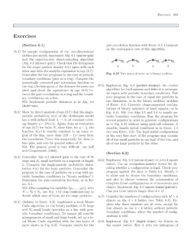
Generalize the two programs to the case of periodic Fig. 6.37 Two types of move on a binary necklace.
boundary conditions (pins on a ring). Compute the
periodically corrected pair correlation function on
the ring (the histogram of the distance between two (6.5) Implement Alg. 6.3 (pocket-binary), the cluster
pins) and check the equivalence in eqn (6.9) be- algorithm for hard squares and disks in a rectangu-
tween the pair correlations on a ring and the bound- lar region with periodic boundary conditions. Test
ary correlations on a line. your program in the case of equal-size particles in
NB: Implement periodic distances as in Alg. 2.6 one dimension, or in the binary necklace problem
(diff-vec). of Exerc. 6.3. Generate phase-separated configu-
rations of binary mixtures of hard squares, as in
(6.2) Show by direct analysis of eqn (6.7) that the single- Fig. 6.14. NB: Use Algs 2.5 and 2.6 to handle pe-
particle probability π(x) of the clothes-pin model riodic boundary conditions. Run the program for
has a well-defined limit L →∞ at constant cover- several minutes in order to generate configurations
ing density η =2Nσ/L. Again, from an evaluation as in Fig. 6.10 without using grid/cell schemes. If
1
of eqn (6.7) for finite N, show that, for η< ,the possible, handle initial conditions as in Exerc. 1.3
2
function π(x) is exactly constant in an inner re- (see also Exerc. 2.3). The legal initial configuration
gion of the line, more than (2N − 1)σ away from at the very first start of the program may contain
the boundaries. Prove this analytically for three or all of the small particles in one half of the box, and
four pins, and also for general values of N. all of the large particles in the other.
NB: The general proof is very difficult—see Leff
and Coopersmith (1966).
(Section 6.2)
(6.3) Generalize Alg. 6.2 (direct-pin)to the case of N l
large and N s small particles on a segment of length (6.6) Implement Alg. 6.4 (naive-dimer)on a 4×4square
L. Compute the single-particle probability distri- lattice. Use an occupation-number vector for de-
bution π(x) for the large particles. Generalize the ciding whether a configuration is legal. Check your
program to the case of particles on a ring with pe- program against the data in Table 6.2. Modify it
riodic boundary conditions (a “binary necklace”). to allow you to choose the boundary conditions,
Determine the pair-correlation function, as in Ex- and also to choose between the enumeration of
erc. 6.1. complete dimer configurations or of monomers and
NB: After sampling the variables {y 1,...,y N },with dimers. Implement Alg. 6.5 (naive-dimer(patch)).
N = N l + N s, use Alg. 1.12 (ran-combination)to Can you treat lattices larger than 4 × 4?
decide which ones of them are the large particles. (6.7) Consider the numbers of configurations with M> 0
dimers on the 4 × 4 lattice (see Table 6.2). Ex-
(6.4) (Relates to Exerc. 6.3). Implement a local Monte
plain why these numbers are all even, except for
Carlo algorithm for the binary necklace of N l large
four dimers on the 4 × 4 lattice without periodic
and N s small beads (particles on a line with peri-
odic boundary conditions). To sample all possible boundary conditions, where the number of config-
urations is odd.
arrangements of small and large beads, set up a lo-
cal Monte Carlo algorithm with the two types of (6.8) Implement Alg. 6.7 (depth-dimer) for dimers on
move shown in Fig. 6.37. Compare results for the the square lattice. Test it with the histogram of