Page 323 -

310 Dynamic Monte Carlo methods

7.1.1 Faster-than-the-clock algorithms

Indynamic Monte Carlo methods, as in equilibriummethods, algorithm
design does notstop with naive approaches.Inthe late stages of Alg. 7.1
(naive-deposition),most deposition attempts are rejected and do not
change the configuration.This indicates that better methods can be
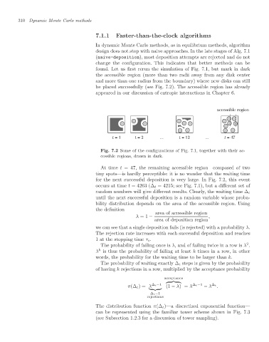
found.Let usfirst rerunthe simulation of Fig. 7.1,but mark in dark
the accessibleregion (more than two radii away fromany disk center
and more than one radiusfromthe boundary) where new disks can still
be placed successfully (see Fig. 7.2). The accessibleregionhas already
appeared in ourdiscussion ofentropic interactions in Chapter 6.

accessible region

t = 1 t = 2 ... t = 12 ... t = 47

Fig. 7.2 Some of the configurations of Fig. 7.1, together with their ac-
cessible regions, drawn in dark.

Attime t = 47, the remaining accessibleregion—composed oftwo
tiny spots—is hardly perceptible: it is nowonder that the waiting time
for the nextsuccessful depositionis verylarge.In Fig. 7.2, this event
occurs at time t = 4263 (∆ t = 4215; see Fig. 7.1),buta different set of
randomnumbers will givedifferent results. Clearly,the waiting time ∆ t
until the nextsuccessful depositionis a random variable whose proba-
bility distribution depends onthe area of the accessibleregion.Using
the definition
area of accessibleregion
λ =1 − ,
area ofdepositionregion
we can see that a singledepositionfails (is rejected)with a probability λ.
The rejection rate increases witheachsuccessful deposition and reaches
1 at the stopping time τ s .
2
The probabilityoffailing once is λ,and offailing twice in a row is λ .
k
λ is thus the probabilityoffailing at least k times in a row,in other
words, the probability forthe waiting time to be larger than k.
The probabilityof waiting exactly ∆ t stepsisgiven by the probability
ofhaving k rejections in a row,multiplied by the acceptance probability

acceptance

π(∆ t )= λ ∆ t −1 (1 − λ)= λ ∆ t −1 − λ ∆ t .

∆ t −1
rejections
The distributionfunction π(∆ t )—a discretized exponential function—
can be represented using the familiar tower scheme shownin Fig. 7.3
(see Subsection 1.2.3 foradiscussion oftower sampling).