Page 48 -

1.2 Basic sampling 35

1.2.4 Continuous distributions and sample
transformation

The two discrete methods of Subsection 1.2.3 remain meaningful in the
continuum limit.For the rejectionmethod, the arrangement ofboxes in
Fig.1.28 simply becomes a continuouscurve π(x) in some range x min <
x< x max (see Alg.1.16 (reject-continuous)). Weshall often use a
refinement ofthis simple scheme, where the function π(x), which we
want to sample, is compared not with a constant function π max but with
another function ˜π(x) that weknow how to sample, and is everywhere
larger than π(x)(see Subsection2.3.4).

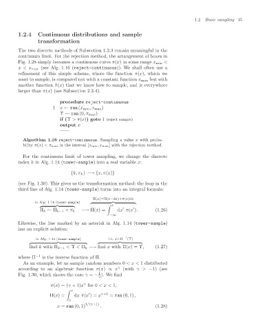
procedure reject-continuous
1 x ← ran(x min ,x max )
Υ ← ran (0,π max)
if (Υ >π(x)) goto 1 (reject sample)
output x
——
Algorithm 1.16 reject-continuous. Sampling a value x with proba-
bility π(x) <π max in the interval [x min,x max] with the rejection method.

Forthe continuum limit oftower sampling, we change the discrete
index k in Alg.1.14 (tower-sample) into arealvariable x:

{k, π k }−→ {x, π(x)}
(see Fig. 1.30). This gives usthe transformationmethod: the loopinthe
third line of Alg.1.14 (tower-sample) turns into an integral formula:
Π(x)=Π(x−dx)+π(x)dx
in Alg. 1.14 (tower-sample)
x

−→ Π(x)= dx π(x ) . (1.26)

Π k ← Π k−1 + π k
−∞
Likewise, the line marked by an asterisk in Alg.1.14 (tower-sample)
has an explicit solution:
in Alg. 1.14 (tower-sample) i.e. x=Π −1 (Υ)

find k with Π k−1 < Υ < Π k −→ find x with Π(x)= Υ, (1.27)
where Π −1 is the inverse function of Π.
Asan example, let ussamplerandomnumbers 0 <x< 1 distributed
according to an algebraic function π(x) ∝ x γ (with γ> −1) (see
1
Fig.1.30, which showsthe case γ = − ). We find
2
γ
π(x)=(γ +1)x for 0 <x < 1,

x

Π(x)= dxπ(x )= x γ+1 = ran(0, 1) ,
0
1/(γ+1)
x = ran(0, 1) . (1.28)