Page 108 - The Combined Finite-Discrete Element Method

SCREENING CONTACT DETECTION ALGORITHM 91

−1 −1 −1 −1 −1 −1 −1 −1 −1 −1
 
 −1 −1 −1 −1 −1 −1 9 −1 −1 −1 
 
 −1 −1 −1 −1 −1 −1 −1 −1 −1 −1 
 
 −1 −1 −1 −1 −1 −1 −1 −1 −1 −1 
 −1 −1 −1 −1 −1 6 4 −1 −1 −1 


(3.31)
 −1 −1 −1 −1 −1 8 −1 −1 −1 −1 

C = 
 
 −1 −1 −1 −1 −1 −1 −1 −1 −1 −1 
 
 −1 −1 −1 −1 −1 −1 −1 −1 −1 −1 
−1 −1 −1 −1 −1 −1 −1 −1 −1 −1
 
−1 −1 −1 −1 −1 −1 −1 −1 −1 −1
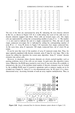
The rest of the lists are represented by array E, indicating the next discrete element
in the list, as shown in Figure 3.20. It is worth noting that most of the cells have no
discrete elements mapped onto them. These cells are termed empty cells. The empty
cells are represented by setting the corresponding number of array C to −1. The number
−1 is also used to indicate the end of a singly connected list. Thus, the end of each
singly connected non-empty list is indicated by setting the corresponding number of
array E to −1. Array E shown in Figure 3.20 represents four singly connected lists.
At the same time, array C represents 100 singly connected lists, out of which 96 are
empty.
It can be seen that most of the numbers of array C represent empty lists. Thus, for
space sparsely populated with discrete elements, array C may be very large. This is the
reason for calling the algorithm the screen array algorithm. Array C ‘screens’ discrete
elements into correct cells.
However, in situations where discrete elements are closely packed together, such as
packing problems, most of the cells are not empty. In such cases, this algorithm makes
sense. Otherwise, the RAM space needed to store array C may not always be available, or
alternatively, the size of the problem (total number of discrete elements) may be limited
by the available RAM space if expensive operations such as memory paging are to be
avoided (see Chapter 9). Array C is a two-dimensional array. In 3D space it is a three-
dimensional array. Accessing elements of such an array requires multiplication. Thus, in

8

6
Integer array E 4 2 1

9 7 5 3

−1 1 −1 2 3 −1 5 −1 7
1 2 3 4 5 6 7 8 9
Head = 4, i.e. Head = 6, i.e. Head = 8, i.e. Head = 9, i.e.
C[5][7] = 4 C[5][6] = 6 C[6][6] = 8 C[2][7] = 9

Figure 3.20 Singly connected lists for discrete elements system shown in Figure 3.19.