Page 944 - The Mechatronics Handbook

0066_frame_C31.fm Page 7 Friday, January 18, 2002 5:51 PM

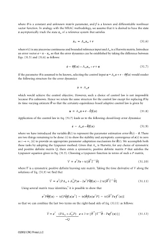
where θ is a constant and unknown matrix parameter, and f is a known and differentiable nonlinear
vector function. In analogy with the MRAC methodology, we assume that it is desired to have the state
x asymptotically track the state x m of a reference system that satisfies

x ˙ m = A m x m + r (31.6)

where r(t) is any piecewise continuous and bounded reference input and A m is a Hurwitz matrix. Introduce
an error vector e = x − x m so that the error dynamics can be established by taking the difference between
Eqs. (31.5) and (31.6) as follows:

e ˙ = θfx() A m x m – r + u (31.7)
–
If the parameter θ is assumed to be known, selecting the control input u = A m x + r − θf(x) would render
the following structure for the error dynamics:

e ˙ = A m e

which would achieve the control objective. However, such a choice of control law is not impossible
because θ is unknown. Hence we retain the same structure for the control law except for replacing θ by
θ
ˆ
its time-varying estimate so that the certainty-equivalence-based adaptive control law is given by
u = A m x + r θ fx() (31.8)
ˆ
–
Application of the control law in Eq. (31.7) leads us to the following closed-loop error dynamics:
e ˙ = A m e θfx() (31.9)
˜
–
ˆ
θ
θ
˜
where we have introduced the variable (t) to represent the parameter estimation error (t) − θ. There
are two things remaining to be done: (i) to show the stability and asymptotic convergence of e(t) to zero
ˆ
as t → ∞, (ii) to provide an appropriate parameter adaptation mechanism for (t). We accomplish bothθ
these tasks by adopting the Lyapunov method. Given that A m is Hurwitz, for any choice of symmetric
and positive definite matrix Q, there exists a symmetric, positive definite matrix P that satisfies the
Lyapunov equation given in Eq. (31.3). Choosing a Lyapunov function in terms of such a P matrix,
V = e Pe + tr θ Γ θ] (31.10)
T
[
˜
T
–
˜
1
where Γ is a symmetric positive definite learning rate matrix. Taking the time derivative of V along the
solutions of Eq. (31.9) we find that
V = e PA m +( A m P)e 2e Pθfx() + 2 tr θ Γ θ[ ˜ T – 1 ˙ ˜ ] (31.11)
T
T
˙
T
˜
–
9
Using several matrix trace identities, it is possible to show that
T
T
˜
[
[
T
e Pθfx() = tr Pθfx()e ] = tr θ fx()e P] = tr θ Pef x()]
T
T
[
˜
˜
˜
so that we can combine the last two terms on the right-hand side of Eq. (31.11) as follows:
1 ˙
˜
V = e T ( PA m + A m P) e + 2 tr θ { Γ θ – Pef x()}] (31.12)
T
[
T
T
˙
–
˜
      
– Q
©2002 CRC Press LLC