Page 287 - Thermal Hydraulics Aspects of Liquid Metal Cooled Nuclear Reactors

Large-eddy simulation: Application to liquid metal fluid flow and heat transfer 257

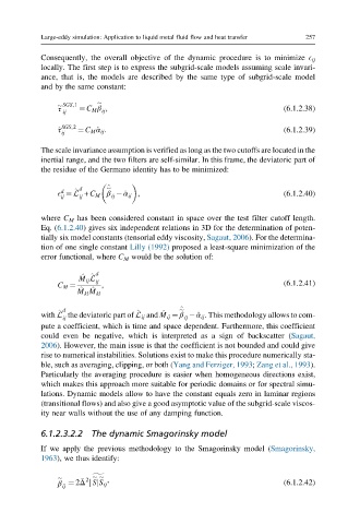
Consequently, the overall objective of the dynamic procedure is to minimize E ij
locally. The first step is to express the subgrid-scale models assuming scale invari-
ance, that is, the models are described by the same type of subgrid-scale model
and by the same constant:

SGS,1
τ ¼ C M β , (6.1.2.38)
ij ij
^ τ SGS,2 ¼ C M ^ α ij : (6.1.2.39)
ij
The scale invariance assumption is verified as long as the two cutoffs are located in the
inertial range, and the two filters are self-similar. In this frame, the deviatoric part of
the residue of the Germano identity has to be minimized:
^
d
^
d
E ¼ L + C M β ^ α ij , (6.1.2.40)
ij ij ij
where C M has been considered constant in space over the test filter cutoff length.
Eq. (6.1.2.40) gives six independent relations in 3D for the determination of poten-
tially six model constants (tensorial eddy viscosity, Sagaut, 2006). For the determina-
tion of one single constant Lilly (1992) proposed a least-square minimization of the
error functional, where C M would be the solution of:

^ ^ d
M ij L ij
C M ¼ , (6.1.2.41)
^ ^
M kl M kl
d
^
^
^
^
with L the deviatoric part of L ij and M ij ¼ β ^ α ij . This methodology allows to com-
ij
ij
pute a coefficient, which is time and space dependent. Furthermore, this coefficient
could even be negative, which is interpreted as a sign of backscatter (Sagaut,
2006). However, the main issue is that the coefficient is not bounded and could give
rise to numerical instabilities. Solutions exist to make this procedure numerically sta-
ble, such as averaging, clipping, or both (Yang and Ferziger, 1993; Zang et al., 1993).
Particularly the averaging procedure is easier when homogeneous directions exist,
which makes this approach more suitable for periodic domains or for spectral simu-
lations. Dynamic models allow to have the constant equals zero in laminar regions
(transitional flows) and also give a good asymptotic value of the subgrid-scale viscos-
ity near walls without the use of any damping function.
6.1.2.3.2.2 The dynamic Smagorinsky model

If we apply the previous methodology to the Smagorinsky model (Smagorinsky,
1963), we thus identify:

2 g ,
β ¼ 2Δ j SjS ij (6.1.2.42)
ij