Page 38 - Thermodynamics of Biochemical Reactions

32 Chapter 2 Structure of Thermodynamics

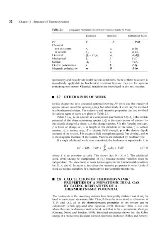
Table 2.1. Conjugate Properties Involved in Various Kinds of Work

Extensive Intensive Differential Work
PV V -P -PdV
Chemical
non rx system ni Pi Pidni
rx system nci Pi Pi dnci
Electrical Qi = Fzini 4i 4; dQi
Mechanical L .f .f dL
Surface AS 7 dAs
Electric polarization P E E dP
Magnetic polarization m B B dm

spontaneity and equilibrium under various conditions. None of these equations is
immediately applicable to biochemical reactions because they are for systems
containing one species. Chemical reactions are introduced in the next chapter.

2.7 OTHER KINDS OF WORK

In this chapter we have discussed systems involving PV work and the transfer of
species into or out of the system (pi dn,), but other kinds of work may be involved
in a biochemical system. The extensive and intensive properties that are involved
in various types of work are given in Table 2.1.
Table 2.1, nCi is the amount of a component (see Section 3.3), qhi is the electric
potential of the phase containing species i, Qi is the contribution of species i to
the electric charge of a phase, zi is the charge number, F is the Faraday constant,
,f is force of elongation, L is length in the direction of the force, 7 is surface
tension, A, is surface area, E is electric field strength, p is the electric dipole
moment of the system, B is magnetic field strength (magnetic flux density), and rn
is the magnetic moment of the system. Vectors are indicated by boldface type.
If a single additional work term is involved, the fundamental equation for U is
dU = TdS - VdP + NS pidn, + XdY (2.7-1)

i= 1
where Y is an extensive variable. This shows that D = N, + 3. The additional
work terms should be independent of (ni} because natural variables must be
independent. The same form of work terms appear in the fundamental equations
for H, A, and G. In order to introduce the intensive properties in other kinds of
work as natural variables, it is necessary to use Legendre transforms.

2.8 CALCULATION OF THERMODYNAMIC
PROPERTIES OF A MONATOMIC IDEAL GAS
BY TAKING DERIVATIVES OF A
THERMODYNAMIC POTENTIAL

The treatments in the preceding sections have been pretty abstract, and it may be
hard to understand statements like: Thus, if G can be determined as a function of
T P, and {nil, all of the thermodynamic properties of the system can be
calculated” (which appeared after equation 2.5-9). However, there is one case
where this can be demonstrated in detail, and that is for a monatomic ideal gas
(Greiner, Neise, and Stocker, 1995). Statistical mechanics shows that the Gibbs
energy of a monatomic ideal gas without electronic excitation (Silbey and Alberty,