
Page 145 - Bird R.B. Transport phenomena
P. 145
§4.3 Flow of Inviscid Fluids by Use of the Velocity Potential 129
Hence the stream function is
ф(х, у) = -v y[ 1 - - ^ — ^ (4.3-18)
x
V xr + yV
To make a plot of the streamlines it is convenient to rewrite Eq. 4.3-18 in dimensionless form
, Y) = -Y( 1 - —r^—-) (4.3-19)
2
V X 2 + Y /
in which ^ = ф/v^R, X = x/R, and Y = y/R.
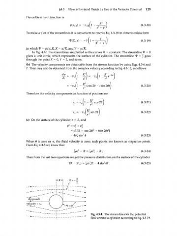
In Fig. 4.3-1 the streamlines are plotted as the curves У = constant. The streamline 4? = 0
gives a unit circle, which represents the surface of the cylinder. The streamline ^ = § goes
through the point X = 0, Y = 2, and so on.
(b) The velocity components are obtainable from the stream function by using Eqs. 4.3-6 and
7. They may also be obtained from the complex velocity according to Eq. 4.3-12, as follows:
t —
= - i d 1 - ^ ( c o s 2 0 - l s i n 20) (4.3-20)
Therefore the velocity components as function of position are
/ »2 \
v x = v x V 1 - ^ r 2 cos 26) (4.3-21)
/
r
\
(4.3-22)
(c) On the surface of the cylinder, r = R, and
v 1 = v\ + v]
2
1
= i£[(l - cos 26>) + (sin 20) ]
= Avi sin 2 в (4.3-23)
When 0 is zero or тг, the fluid velocity is zero; such points are known as stagnation points.
From Eq. 4.3-5 we know that
\pv 2 + <3> = \pvl + <3> x (4.3-24)
Then from the last two equations we get the pressure distribution on the surface of the cylinder
2
& - ®J = lpvi(l - 4 sin в) (4.3-25)
Fig. 4.3-1. The streamlines for the potential
flow around a cylinder according to Eq. 4.3-19.