
Page 188 - Bird R.B. Transport phenomena
P. 188
172 Chapter 5 Velocity Distributions in Turbulent Flow
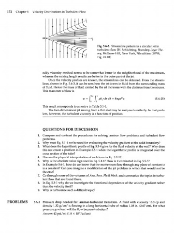
Fig. 5.6-3. Streamline pattern in a circular jet in
turbulent flow [H. Schlichting, Boundary-Layer The-
ory, McGraw-Hill, New York, 7th edition (1979),
Fig. 24.10].
eddy viscosity method seems to be somewhat better in the neighborhood of the maximum,
whereas the mixing length results are better in the outer part of the jet.
Once the velocity profiles are known, the streamlines can be obtained. From the stream-
lines, shown in Fig. 5.6-3, it can be seen how the jet draws in fluid from the surrounding mass
of fluid. Hence the mass of fluid carried by the jet increases with the distance from the source.
This mass rate of flow is
w = pv zr dr de = 8TTP*/°Z (5.6-25)
This result corresponds to an entry in Table 5.1-1.
The two-dimensional jet issuing from a thin slot may be analyzed similarity. In that prob-
lem, however, the turbulent viscosity is a function of position.
QUESTIONS FOR DISCUSSION
1. Compare and contrast the procedures for solving laminar flow problems and turbulent flow
problems.
2. Why must Eq. 5.1-4 not be used for evaluating the velocity gradient at the solid boundary?
3. What does the logarithmic profile of Eq. 5.3-4 give for the fluid velocity at the wall? Why does
this not create a problem in Example 5.5-1 when the logarithmic profile is integrated over the
cross section of the tube?
4. Discuss the physical interpretation of each term in Eq. 5.2-12.
5. Why is the absolute value sign used in Eq. 5.4-4? How is it eliminated in Eq. 5.5-5?
6. In Example 5.6-1, how do we know that the momentum flow through any plane of constant z
is a constant? Can you imagine a modification of the jet problem in which that would not be
the case?
7. Go through some of the volumes oi Ann. Revs. Fluid Mech. and summarize the topics in turbu-
lent flow that are found there.
8. In Eq. 5.3-1 why do we investigate the functional dependence of the velocity gradient rather
than the velocity itself?
9. Why is turbulence such a difficult topic?
PROBLEMS 5A.1 Pressure drop needed for laminar-turbulent transition. A fluid with viscosity 18.3 cp and
density 1.32 g/cm 3 is flowing in a long horizontal tube of radius 1.05 in. (2.67 cm). For what
pressure gradient will the flow become turbulent?
5
Answer: 42 psi/mi (1.8 X 10 Pa/km)