Page 388 - Bird R.B. Transport phenomena

370 Chapter 11 The Equations of Change for Nonisothermal Systems

(a) Simplify the equations of continuity, motion, and energy according to the postulates:
2
2
2
v = b v (x, y), d v /dy 2 « d v /dx , and T = T{y). These postulates are reasonable for slow
z
z z
z
flow, except near the edges у = ± Wand z = ±H.
(b) List the boundary conditions to be used with the problem as simplified in (a).
(c) Solve for the temperature, pressure, and velocity profiles.
(d) When making diffusion measurements in closed chambers, free convection can be a seri-
ous source of error, and temperature gradients must be avoided. By way of illustration, com-
pute the maximum tolerable temperature gradient, A, for an experiment with water at 20°C in
a chamber with В = 0.1 mm, W = 2.0 mm, and H = 2 cm, if the maximum permissible convec-
tive movement is 0.1% of_H in a one-hour experiment.
2
3
Answers: (c) vXx, y) = ^ — (x - B )y; (d) 2.7 X 10~ K/cm
2
11C.3. Tangential annular flow of a highly viscous liquid. Show that Eq. 11.4-13 for flow in an an-
nular region reduces to Eq. 10.4-9 for plane slit flow in the limit as к approaches unity. Com-
parisons of this kind are often useful for checking results.
The right side of Eq. 11.4-13 is indeterminate at к = 1, but its limit as к —» 1 can be ob-
tained by expanding in powers of s = 1 - к. To do this, set к = 1 - ^ and f = 1 — s[\ -
(x/b)]; then the range к < f < 1 in Problem 11.4-2 corresponds to the range 0 < x < fr in §10.4.
After making the substitutions, expand the right side of Eq. 11.4-13 in powers of e (neglecting
terms beyond в ) and show that Eq. 10.4-9 is obtained.
2
11C.4. Heat conduction with variable thermal conductivity.
(a) For steady-state heat conduction in solids, Eq. 11.2-5 becomes (V • q) = 0, and insertion of
Fourier's law gives (V • kVT) = 0. Show that the function F = JkdT + const, satisfies the
Laplace equation VF = 0, provided that k depends only on T.
2
(b) Use the result in (a) to solve Problem 10B.12 (part a), using an arbitrary function k(T).
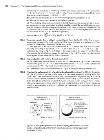
11C.5. Effective thermal conductivity of a solid with spherical inclusions (Fig. 11C.5). Derive Eq.
9.6-1 for the effective thermal conductivity of a two-phase system by starting with Eqs.
1 IB.8-1 and 2. We construct two systems both contained within a spherical region of radius
R: f (a) the "true" system, a medium with thermal conductivity k , in which there are embed-
Q
ded n tiny spheres of thermal conductivity k and radius R; and (b) an "equivalent" system,
x
which is a continuum, with an effective thermal conductivity k . Both of these systems are
eff
placed in a temperature gradient A, and both are surrounded by a medium with thermal
conductivity /c. 0

Medium 0 with Medium 0 with
thermal conductivity k 0 thermal conductivity /c 0
Medium 0 Sphere of radius
n spheres of
material 1 R' of a hypothetical
of radius R "smoothed out"
and thermal material equivalent
conductivity k^ to the granular
material in (a)

Sphere of radius R' Thermal conductivity is A: eft

(a) (b)
Fig. 11C.5. Thought experiment used by Maxwell to get the thermal conductiv-
ity of a composite solid: (a) the "true" discrete system, and (b) the "equivalent"
continuum system.