Page 398 - Bird R.B. Transport phenomena

380 Chapter 12 Temperature Distributions with More Than One Independent Variable

Sf(r) = — — = dimensionless fluid temperature (12.1-42)

£ = ^ = dimensionless radial coordinate (12.1-43)
К
a t
s
т = — = dimensionless time (12.1-44)
R
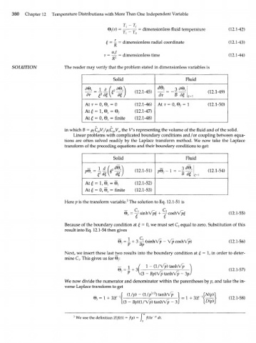
SOLUTION The reader may verify that the problem stated in dimensionless variables is

Solid Fluid

(12.1-45) (12.1-49)
дт В 6
A t T = o, 0 = 0 (12.1-46) Atr = 0,0/ = 1 (12.1-50)
S
(12.1-47)
Atf = o, 0 = finite (12.1-48)
S
in which В = p fC pfVf/p£ psV s, the V's representing the volume of the fluid and of the solid.
Linear problems with complicated boundary conditions and/or coupling between equa-
tions are often solved readily by the Laplace transform method. We now take the Laplace
transform of the preceding equations and their boundary conditions to get:

Solid Fluid
d
— з 0 4
P®s e (12.1-51) В df (12.1-54)
% , - 1
(12.1-52)
AM = = 0, 0,= finite (12.1-53)

Here p is the transform variable. The solution to Eq. 12.1-51 is
3
+ -j cosh Vptj (12.1-55)

Because of the boundary condition at f = 0, we must set C equal to zero. Substitution of this
2
result into Eq. 12.1-54 then gives
® = ^ + 3 ^ (sinhVp - Vp coshVp) (12.1-56)
f
Bp
Next, we insert these last two results into the boundary condition at f = 1, in order to deter-
mine C . This gives us for 0/:
}
-jJ- ^—-\ (12.1-57)
V(3 - Bp)Vp tanhVp - 3p/
We now divide the numerator and denominator within the parentheses by p, and take the in-
verse Laplace transform to get

0, • = 1 + (12.1-58)
(3 - Bp)(l /Vp) tanhVp - 3 [Dip)J

3
We use the definition £{f(t)\ = ~f{p) = f /(Oe"'" dt.