Page 338 - Tunable Lasers Handbook

298 Norman P. Barnes

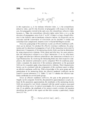
In this expression. tzo is the ordinary refractive index, ne is the extraordinary
refractive index. and e is the direction of propagation with respect to the optic
axis. For propagation normal to the optic axis, the extraordinary refractive index
becomes 11,. Thus. the extraordinary refractive index varies from no to ne as the
direction of propagation vanes from 0' to 90". If there is a large enough differ-
ence in the ordinary and extraordinary refractive indices, the dispersion can be
overcome and the conservation of momentum can be satisfied. A similar, but
somewhat more complicated, situation exists in biaxial birefringent crystals.
Given the point group of the nonlinear crystal. an effective nonlinear coeffi-
cient can be defined. To calculate the effective nonlinear coefficient, the polar-
ization and the direction of propagation of each of the interacting waves must be
determined. Components of the interacting electric fields can then be determined
by using trigonometric relations. If the signal and idler have the same polariza-
tion. the interaction is referred to as a Type I interaction. If, on the other hand,
the signal and idler have different polarizations. the interaction is referred to as a
Type I1 interaction. By resolving the interacting fields into their respective com-
ponents, the nonlinear polarization can be computed. With the nonlinear polar-
ization computed. the projection of the nonlinear polarization on the generated
field can be computed, again using trigonometric relations. These trigonometric
factors can be combined with the components of the nonlinear tensor to define
an effective nonlinear coefficient. With a knowledge of the point group and the
polarization of the interacting fields, the effective nonlinear coefficient can be
found in several references [Ill. Tables 7.2 and 7.3 tabulate the effective non-
linear coefficient for several point groups.
Given an effective nonlinear coefficient, the gain at the generated wave-
lengths can be computed. To do this, the parametric approximation is usually uti-
lized. In the parametric approximation, the amplitudes of the interacting electric
fields are assumed to vary slowly compared with the spatial variation associated
with the traveling waves. At optical wavelengths, this is an excellent approxima-
tion. If, in addition. the amplitude of the pump is nearly constant, the equation
describing the growth of the signal and the idler assumes a particularly simple
form [12-141: