Page 122 - Video Coding for Mobile Communications Efficiency, Complexity, and Resilience

Section 4.3. Di erential Methods 99

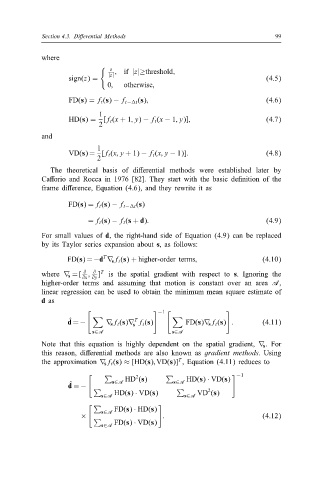
where

z ; if |z |≥threshold;
sign(z )= |z| (4.5)
0; otherwise;

FD(s)= f t (s) − f t −@t (s); (4.6)
1
HD(s)= [f t (x +1;y ) − f t (x − 1;y )]; (4.7)
2
and
1
VD(s)= [f t (x; y +1) − f t (x; y − 1)]: (4.8)
2
The theoretical basis of di erential methods were established later by
Ca orio and Rocca in 1976 [82]. They start with the basic de nition of the
frame di erence, Equation (4.6), and they rewrite it as

FD(s)= f t (s) − f t −@t (s)
= f t (s) − f t (s + d): (4.9)

For small values of d, the right-hand side of Equation (4.9) can be replaced
by its Taylor series expansion about s, as follows:

T
FD(s)= −d ∇ s f t (s) + higher-order terms; (4.10)
@
@ T
where ∇ s =[ ; ] is the spatial gradient with respect to s. Ignoring the
@y
@x
higher-order terms and assuming that motion is constant over an area A,
linear regression can be used to obtain the minimum mean square estimate of
d as

−1
ˆ
T
d = − ∇ s f t (s)∇ f t (s) FD(s)∇ s f t (s) : (4.11)
s
s∈A s∈A
Note that this equation is highly dependent on the spatial gradient, ∇ s . For
this reason, di erential methods are also known as gradient methods. Using
T
the approximation ∇ s f t (s) ≈ [HD(s); VD(s)] , Equation (4.11) reduces to
−1
HD (s) HD(s) · VD(s)
2
ˆ
d = − s∈A s∈A 2

s∈A HD(s) · VD(s) s∈A VD (s)
FD(s) · HD(s)
× s∈A : (4.12)
FD(s) · VD(s)
s∈A