Page 44 - Video Coding for Mobile Communications Efficiency, Complexity, and Resilience

Section 2.5. Video Coding Basics 21

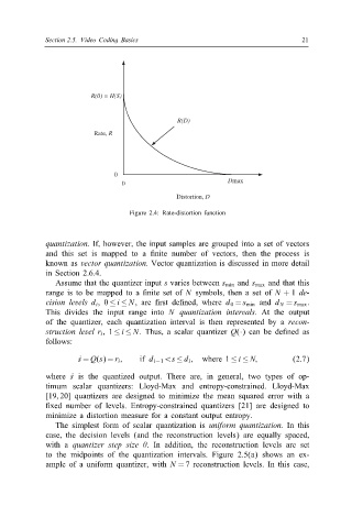
R(0) = H(S)

R(D)
Rate, R

0
0 Dmax
Distortion, D
Figure 2.4: Rate-distortion function

quantization. If, however, the input samples are grouped into a set of vectors
and this set is mapped to a nite number of vectors, then the process is
known as vector quantization. Vector quantization is discussed in more detail
in Section 2.6.4.
Assume that the quantizer input s varies between s min and s max and that this
range is to be mapped to a nite set of N symbols, then a set of N +1 de-
cision levels d i ,0 ≤ i ≤ N , are rst de ned, where d 0 = s min and d N = s max .
This divides the input range into N quantization intervals. At the output
of the quantizer, each quantization interval is then represented by a recon-
struction level r i ,1 ≤ i ≤ N . Thus, a scalar quantizer Q(·) can be de ned as
follows:

s˙= Q(s)= r i ; if d i−1 ¡s ≤ d i ; where 1 ≤ i ≤ N; (2.7)

where s˙ is the quantized output. There are, in general, two types of op-
timum scalar quantizers: Lloyd-Max and entropy-constrained. Lloyd-Max
[19, 20] quantizers are designed to minimize the mean squared error with a
xed number of levels. Entropy-constrained quantizers [21] are designed to
minimize a distortion measure for a constant output entropy.
The simplest form of scalar quantization is uniform quantization. In this
case, the decision levels (and the reconstruction levels) are equally spaced,
with a quantizer step size . In addition, the reconstruction levels are set
to the midpoints of the quantization intervals. Figure 2.5(a) shows an ex-
ample of a uniform quantizer, with N = 7 reconstruction levels. In this case,