Page 60 - Wind Energy Handbook

34 THE WIND RESOURCE

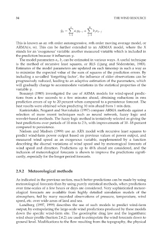
m
n
X X
^ y y k ¼ a i y k i þ b j e k j
i¼1 j¼1
This is known as an nth order autoregressive, mth order moving average model, or
ARMA(n, m). This can be further extended to an ARMAX model, where the X
stands for an ‘exogenous’ variable: another measured variable which is included in
the prediction because it influences y.
The model parameters a i , b j can be estimated in various ways. A useful technique
is the method of recursive least squares, or RLS (Ljung and So ¨derstro ¨m, 1983).
Estimates of the model parameters are updated on each timestep in such a way as
to minimize the expected value of the sum of squares of the prediction errors. By
including a so-called ‘forgetting factor’, the influence of older observations can be
progressively reduced, leading to an adaptive estimation of the parameters, which
will gradually change to accommodate variations in the statistical properties of the
variable y.
Bossanyi (1985) investigated the use of ARMA models for wind-speed predic-
tions from a few seconds to a few minutes ahead, obtaining reductions in rms
prediction errors of up to 20 percent when compared to a persistence forecast. The
best results were obtained when predicting 10 min ahead from 1 min data.
Kariniotakis, Nogaret and Stavrakakis (1997) compare ARMA methods against a
selection of more recent techniques such as neural network, fuzzy logic and
wavelet-based methods. The fuzzy logic method is tentatively selected as giving the
best predictions over periods of 10 min to 2 h, with improvements of 10–18 percent
compared to persistence.
Nielsen and Madsen (1999) use an ARX model with recursive least squares to
predict wind-farm power output based on previous values of power output, and
measured wind speed as an exogenous variable, supplemented by a function
describing the diurnal variations of wind speed and by meteorogical forecasts of
wind speed and direction. Predictions up to 48 h ahead are considered, and the
inclusion of meteorological forecasts is shown to improve the predictions signifi-
cantly, especially for the longer period forecasts.

2.9.2 Meteorological methods

As indicated in the previous section, much better predictions can be made by using
meteorological forecasts than by using purely statistical methods, when predictions
over time-scales of a few hours or days are considered. Very sophisticated meteor-
ological forecasts are available from highly detailed simulation models of the
atmosphere, fed by many recorded observations of pressure, temperature, wind
speed, etc. over wide areas of land and sea.
Landberg (1997, 1999) describes the use of such models to predict wind-farm
output, by extrapolating the large-scale wind predictions produced by these models
down the specific wind-farm site. The geostrophic drag law and the logarithmic
wind shear profile (Section 2.6.2) are used to extrapolate the wind forecasts down to
ground level. Modifications to the flow resulting from the topography, the physical