Page 137 - Characterization and Properties of Petroleum Fractions - M.R. Riazi

QC: IML/FFX
P2: IML/FFX
P1: IML/FFX
AT029-Manual
AT029-Manual-v7.cls
AT029-03
June 22, 2007
3. CHARACTERIZATION OF PETROLEUM FRACTIONS 117
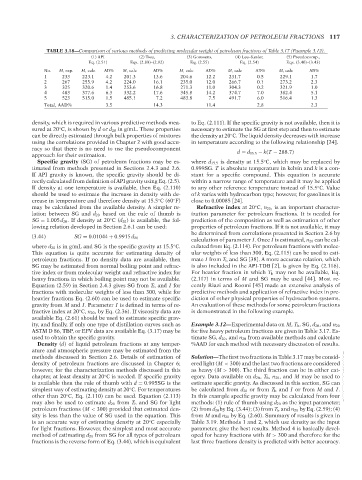
TABLE 3.18—Comparison of various methods of predicting molecular weight of petroleum fractions of Table 3.17 (Example 3.12).
(1) API T1: IML (2) Twu, 14:23 (3) Goossens, (4) Lee–Kesler, (5) Pseudocomp.,
Eq. (2.51) Eqs. (2.89)–(2.92) Eq. (2.55) Eq. (2.54) Eqs. (3.40)–(3.43)
No. M, exp. M, calc AD% M, calc AD% M, calc AD% M, calc AD% M, calc AD%
1 233 223.1 4.2 201.3 13.6 204.6 12.2 231.7 0.5 229.1 1.7
2 267 255.9 4.2 224.0 16.1 235.0 12.0 266.7 0.1 273.2 2.3
3 325 320.6 1.4 253.6 16.8 271.3 11.0 304.3 0.2 321.9 1.0
4 403 377.6 6.3 332.2 17.6 345.8 14.2 374.7 7.0 382.4 5.1
5 523 515.0 1.5 485.1 7.2 483.8 7.5 491.7 6.0 516.4 1.3
Total, AAD% 3.5 14.3 11.4 2.8 2.3
density, which is required in various predictive methods mea- to Eq. (2.111). If the specific gravity is not available, then it is
sured at 20 C, is shown by d or d 20 in g/mL. These properties necessary to estimate the SG at first step and then to estimate
◦
can be directly estimated through bulk properties of mixtures the density at 20 C. The liquid density decreases with increase
◦
using the correlations provided in Chapter 2 with good accu- in temperature according to the following relationship [24].
racy so that there is no need to use the pseudocomponent
approach for their estimation. d = d 15.5 − k(T − 288.7)
Specific gravity (SG) of petroleum fractions may be es- where d 15.5 is density at 15.5 C, which may be replaced by
◦
timated from methods presented in Sections 2.4.3 and 2.6. 0.999SG. T is absolute temperature in kelvin and k is a con-
If API gravity is known, the specific gravity should be di- stant for a specific compound. This equation is accurate
rectly calculated from definition of API gravity using Eq. (2.5). within a narrow range of temperature and it may be applied
If density at one temperature is available, then Eq. (2.110) to any other reference temperature instead of 15.5 C. Value
◦
should be used to estimate the increase in density with de- of k varies with hydrocarbon type; however, for gasolines it is
crease in temperature and therefore density at 15.5 C (60 F) close to 0.00085 [24].
◦
◦
may be calculated from the available density. A simpler re- Refractive index at 20 C, n 20 , is an important character-
◦
lation between SG and d 20 based on the rule of thumb is ization parameter for petroleum fractions. It is needed for
SG = 1.005 d 20 . If density at 20 C(d 20 ) is available, the fol- prediction of the composition as well as estimation of other
◦
lowing relation developed in Section 2.6.1 can be used: properties of petroleum fractions. If it is not available, it may
be determined from correlations presented in Section 2.6 by
(3.44) SG = 0.01044 + 0.9915 d 20
calculation of parameter I. Once I is estimated, n 20 can be cal-
where d 20 is in g/mL and SG is the specific gravity at 15.5 C. culated from Eq. (2.114). For petroleum fractions with molec-
◦
This equation is quite accurate for estimating density of ular weights of less than 300, Eq. (2.115) can be used to esti-
petroleum fractions. If no density data are available, then mate I from T b and SG [38]. A more accurate relation, which
SG may be estimated from normal boiling point and refrac- is also included in the API-TDB [2], is given by Eq. (2.116).
tive index or from molecular weight and refractive index for For heavier fraction in which T b may not be available, Eq.
heavy fractions in which boiling point may not be available. (2.117) in terms of M and SG may be used [44]. Most re-
Equation (2.59) in Section 2.4.3 gives SG from T b and I for cently Riazi and Roomi [45] made an extensive analysis of
fractions with molecular weights of less than 300, while for predictive methods and application of refractive index in pre-
heavier fractions Eq. (2.60) can be used to estimate specific diction of other physical properties of hydrocarbon systems.
gravity from M and I. Parameter I is defined in terms of re- An evaluation of these methods for some petroleum fractions
fractive index at 20 C, n 20 , by Eq. (2.36). If viscosity data are is demonstrated in the following example.
◦
available Eq. (2.61) should be used to estimate specific grav-
ity, and finally, if only one type of distillation curves such as Example 3.12—Experimental data on M, T b , SG, d 20 , and n 20
ASTM D 86, TBP, or EFV data are available Eq. (3.17) may be for five heavy petroleum fractions are given in Table 3.17. Es-
used to obtain the specific gravity. timate SG, d 20 , and n 20 from available methods and calculate
Density (d) of liquid petroleum fractions at any temper- %AAD for each method with necessary discussion of results.
ature and atmospheric pressure may be estimated from the
methods discussed in Section 2.6. Details of estimation of Solution—The first two fractions in Table 3.17 may be consid-
density of petroleum fractions are discussed in Chapter 6; ered light (M < 300) and the last two fractions are considered
however, for the characterization methods discussed in this as heavy (M > 300). The third fraction can be in either cat-
chapter, at least density at 20 C is needed. If specific gravity egory. Data available on d 20 , T b , n 20 , and M may be used to --`,```,`,``````,`,````,```,,-`-`,,`,,`,`,,`---
◦
is available then the rule of thumb with d = 0.995SG is the estimate specific gravity. As discussed in this section, SG can
simplest way of estimating density at 20 C. For temperatures be calculated from d 20 or from T b and I or from M and I.
◦
other than 20 C, Eq. (2.110) can be used. Equation (2.113) In this example specific gravity may be calculated from four
◦
may also be used to estimate d 20 from T b and SG for light methods: (1) rule of thumb using d 20 as the input parameter;
petroleum fractions (M < 300) provided that estimated den- (2) from d 20 by Eq. (3.44); (3) from T b and n 20 by Eq. (2.59); (4)
sity is less than the value of SG used in the equation. This from M and n 20 by Eq. (2.60). Summary of results is given in
is an accurate way of estimating density at 20 C especially Table 3.19. Methods 1 and 2, which use density as the input
◦
for light fractions. However, the simplest and most accurate parameter, give the best results. Method 4 is basically devel-
method of estimating d 20 from SG for all types of petroleum oped for heavy fractions with M > 300 and therefore for the
fractions is the reverse form of Eq. (3.44), which is equivalent last three fractions density is predicted with better accuracy.

Copyright ASTM International
Provided by IHS Markit under license with ASTM Licensee=International Dealers Demo/2222333001, User=Anggiansah, Erick
No reproduction or networking permitted without license from IHS Not for Resale, 08/26/2021 21:56:35 MDT