Page 158 - Introduction to Statistical Pattern Recognition

140 Introduction to Statistical Pattern Recognition

Procedure Ill to find s (the holdout method):

(1) Divide the available samples into two groups: one is called the
design sample set, and the other is called the test sample set.
(2) Using the design samples, follow steps (1)-(4) of Procedure I1 to
find the V and v, for a given s.
(3) Using V and v, found in step (2), classify the test samples by
(4.18), and count the number of misclassified samples.
(4) Change s from 0 to 1, and plot the error vs. s.
In order to confirm the validity of Procedure 111, the following experi-
ment was conducted.

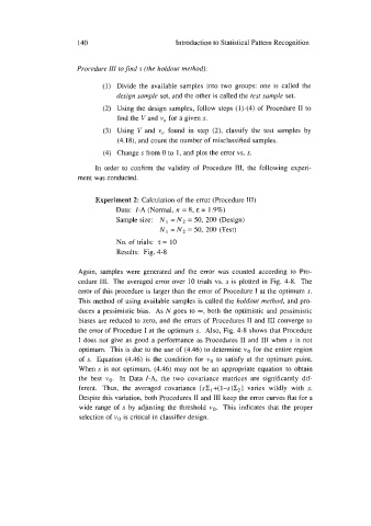
Experiment 2: Calculation of the error (Procedure 111)
Data: I-A (Normal, n = 8, E = 1.9%)
Sample size: N, = N2 = 50, 200 (Design)
N, = N, = 50, 200 (Test)
No. of trials: z = 10
Results: Fig. 4-8

Again, samples were generated and the error was counted according to Pro-
cedure 111. The averaged error over 10 trials vs. s is plotted in Fig. 4-8. The
error of this procedure is larger than the error of Procedure I at the optimum s.
This method of using available samples is called the holdout method, and pro-
duces a pessimistic bias. As N goes to =, both the optimistic and pessimistic
biases are reduced to zero, and the errors of Procedures I1 and I11 converge to
the error of Procedure I at the optimum s. Also, Fig. 4-8 shows that Procedure
I does not give as good a performance as Procedures I1 and I11 when s is not
optimum. This is due to the use of (4.46) to determine vo for the entire region
of s. Equation (4.46) is the condition for vo to satisfy at the optimum point.
When s is not optimum, (4.46) may not be an appropriate equation to obtain
the best yo. In Data I-A, the two covariance matrices are significantly dif-
ferent. Thus, the averaged covariance [sXI+(l-s)Xz] varies wildly with s.
Despite this variation, both Procedures I1 and I11 keep the error curves flat for a
wide range of s by adjusting the threshold VO. This indicates that the proper
selection of vo is critical in classifier design.