Page 242 - Introduction to Statistical Pattern Recognition

224 Introduction to Statistical Pattern Recognition

computation time, the addition of a scalar multiplication is negligibly small.
Thus, we can perform both R and L methods simultaneously within the compu-
tation time needed to conduct the R method alone. In other words, (5.121) and
(5.122) give a simple perturbation equation of the L method from the R method
such that we do not need to design the classifier N times.
The perturbation factor of N,l(Ni-l) is always larger than 1. This
increases (Xi”-k I f(Xi’)--k I ) for an ol -sample, Xi’), and (Xi2)-k2)T
for
(Xi2)-k2) an 02-sample, Xi2). For wI, Xi’) is misclassified if > is satisfied
in (5.121). Therefore, increasing the (Xi1)--h1 )T(Xi’)-k I) term by multiplying
[N1/(Nl-1)I2 means that Xi” has more chance to be misclassified in the L
method than in the R method. The same is true for Xi2) in (5.122). Thus, the
L method gives a larger error than the R method. This is true even if the
classifier of (5.117) is no longer the Bayes. That is, when the distance
classifier of (5.1 17) is used, the L error is larger than the R error regardless of
the test distributions.
,.
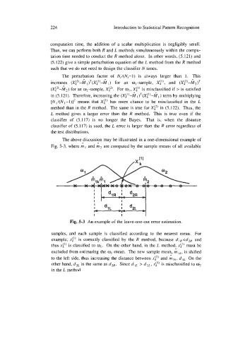
The above discussion may be illustrated in a one-dimensional example of
L.
Fig. 5-3, where m I and m2 are computed by the sample means of all available

I I
I 14 dlR =!= d2R
I I
I - d,L -1- I d2L *
I
I I
Fig. 5-3 An example of the leave-one-out error estimation.

samples, and each sample is classified according to the nearest mean. For
example, xi’) is correctly classified by the R method, because dlR<dZ and
thus xi’) is classified to ol. On the other hand, in the L method, xi!) must be
L.
excluded from estimating the ol -mean. The new sample mean, m Ik, is shifted
to the left side, thus increasing the distance between xi” and A Ik, dlL, On the
other hand, dZL is the same as d,. Since dlL > d2L, xi’) is misclassified to o2
in the L method.